
Abstract
Soil and vegetation carbon stocks play a critical role in human-Earth system models. These stocks (denominated as densities in MgC/ha) affect variables such as land use change emissions and also influence land use change pathways under climate forcing scenarios where terrestrial carbon is assigned a carbon price. Here we present reharmonized soil and vegetation carbon densities both at the 5-arcmin resolution grid cell level and also aggregated to 235 water sheds for 4 land use types (Cropland, Grazed land, Urban land and unmanaged vegetation) and 15 unmanaged land cover types. Moreover, we use the distribution of carbon within and across pixels to define statistical “states” of carbon, once again differentiated by land type. These statistical states are used to define a range of possible carbon values that can be used for defining initial conditions of soil and vegetation carbon in human-Earth system models. We implement these data in a state-of-the-art multi sector dynamics model, namely the Global Change Analysis Model (GCAM), and show that these new data improve several land use responses, especially when terrestrial carbon is assigned a carbon price.
Background & Summary
Global and regional models such as Multisector dynamics models (MSDs) and Integrated human-Earth system (IHES) models are routinely used to assess alternative socio-economic, land use and energy transition pathways1. MSD and IHES models are in the same family of models but have one key difference. MSD models tend to be more economic in nature and lacking in the representation of biophysical processes (e.g. agriculture land use is well represented but the nitrogen cycle is not). IHES models generally are more representative of these biophysical processes through coupling the MSD model with finer resolution land models. As a simple example, GCAM is an MSD model1 (Binsted et al.2) while GCAM when coupled with a detailed land model like GLM (under the GCAM-E3SM framework) represents an IHES model (Calvin et al.3). These models also examine interactions between natural systems (e.g. land, water systems) and human systems (food and energy demand). Soil and vegetation carbon densities play a critical role in these models by influencing the productivity of and profitability from land types (e.g., forest yields, pasture yields, and crop yields) and land use change emissions. Moreover, these densities affect land use change pathways under climate forcing scenarios and low carbon transition scenarios implemented in these models4,5.
IHES, MSD models and economic models generally need to be calibrated with specific carbon densities to initialize the carbon cycle since these models cannot simulate carbon densities through use of spin ups similar to process based earth system models (e.g. Community Land Model or CLM). Note that we define the term “densities” as the stock of carbon denominated in mg/ha, which has already been normalized to bulk density. This term is distinct from the bulk density which is a volumetric term. We also note that the data on carbon densities is also useful for models other than the above mentioned IHES, MSD models (as an example, the Global Trade Analysis Project which utilizes a CGE framework is also calibrated with data from the FAO HWSD compiled by Gibbs, Yui et al.6, aggregated to the GTAP AEZ boundaries (Aguiar et al.7). Land use focused models such as the Global Biosphere Management Model (GLOBIOM) also make use of emissions factors from the IPCC in addition to fine resolution data on carbon stocks to estimate carbon emissions from land use change (Frank et al.8). SI Table 4 shows the carbon inputs used by different models for initializing the carbon cycle for both soil and vegetation carbon. Another challenge is that these models need to be initialized with densities that represent long term potential maximum carbon values since these values are used to spin-up the model in historical years. Thus, carbon densities are used in these models to spin up the historical carbon cycle (e.g. 1700–2015) and model future land use change emissions (e.g. 2016–2100). There have been efforts to reconstruct long term potential carbon densities for soil and vegetation which can inform such calibration efforts. These studies have found that the long term potential carbon densities are much higher than the contemporary values due to ongoing land use and cover change9,10.Moreover, studies have also highlighted difficulties in estimating long term potential carbon densities, since these estimations require long spin up periods themselves11.
To address the above issues, models currently make use of carbon density data that are differentiated by land type but are not always spatially explicit. These carbon densities are often representative of undisturbed land, and thus represent a long-term potential maximum. For example, models have previously used estimates of carbon values on undisturbed land from Houghton et al. Houghton12 and the IPCC13, among others for initialization of the carbon cycle. But these data not being spatially explicit/differentiated often lead to over and underestimation of carbon sequestration potentials, especially in future land use scenarios.
Recently, spatially explicit contemporary data on soil and vegetation carbon data have become available. For example, soil carbon density data have been made available by the FAO14 at a 1 km resolution and at 250 m resolution by the SoilGrids team at the International Soil Reference and Information Centre (ISRIC)15,16. Use of spatially distinct, fine resolution data such as these has the potential to significantly improve results from global and regional models by better capturing the geographies of soil and vegetation carbon stocks17. Even though these data represent contemporary carbon, they can be used to derive potential maximum carbon values that are spatially explicit. However, these carbon data need to be transformed significantly to be used in a robust manner by regional and global models. This is because each of these fine resolution datasets utilizes its own assumptions of land use and land cover which may be distinct from the land use and land cover definitions used by the models in question. For example, many of these fine resolution data use land cover definitions from the European Space Agency Climate Change Initiative (ESA CCI) dataset18,19 while models may use land use definitions from the Historical Database of the Global Environment (HYDE) dataset20 and/or land cover definitions from the Moderate Resolution Imaging Spectrometer (MODIS)21,22. Resolution mismatch between data and models provides an additional challenge. The new, spatially distinct carbon densities are available at a very fine resolution (250 m / 300 m) while models are often configured to use coarser data that better match their working resolution. For example, consistent land datasets that have frequently been used for climate modelling are available at a resolution of 5 arcmins (i.e. ~10 km at the equator)23, and many regional models operate on land units defined by geopolitical and/or geophysical boundaries (See descriptions above for GTAP and GLOBIOM) (Aguiar et al.7, Frank et al.8). Given the difference in resolutions, and the above-mentioned differences in land classifications, a harmonization method is required to appropriately match the fine resolution carbon data with the appropriate land uses and land cover types within a model (as a simple example, a method is required to assign forest carbon correctly to forest portion of pixels, grass carbon to grass portion pixels and that this occurs across the three pools- soil carbon, above ground biomass and below ground biomass). To our knowledge, there is no custom dataset or consistent method that is representative of spatially explicit carbon which can be used to calibrate the carbon cycle in the above mentioned global and regional models.
To address the above limitations, we prepare and present a harmonized dataset of fine resolution organic carbon densities for soil and vegetation biomass to initialize the carbon cycle in IHES and MSD models. The soil data are based on the 250 m-resolution SoilGrids dataset and represent a depth of 0–30 cm (topsoil carbon)16. While multiple depths of soil carbon data are available (e.g. 30 cm -200 cm), we use the depth of 0–30 cm which refers to topsoil carbon since most regional models only make use of carbon stock data at this depth. We note that our programmatic method can produce soil carbon data at different depths if required. These original soil carbon data from the SoilGrids dataset are denominated in MgC of soil carbon per hectare and are derived from several soil properties including the bulk density, clay content, sand and silt content. The aboveground and below ground carbon data are based on the 300 m-resolution Spawn et al. biomass dataset24. The harmonization process associates spatially-explicit carbon densities with specific land types to avoid errors due to mismatches in land type distributions between carbon data and models. For example, the carbon data in a given pixel may be associated with forest, but the model considers this pixel as grassland. The harmonized data associates pixel level carbon with its appropriate land type such that it can be aggregated appropriately to model land types and grids. As a simple example Forest carbon is correctly assigned to forest portion of pixels, grass carbon is assigned to grass portion of pixels and we ensure that this occurs across the three pools- soil carbon, above ground biomass and below ground biomass.
We implemented this carbon reharmonization programmatically in the Moirai land data system25, which can be used to update the data, validate the data (e.g. generating fine resolution and tabular data which can be compared to other sources), define alternate land unit boundaries (e.g., water basins or agro-ecological zones), and harmonize the source carbon data with a generic land type distribution at coarser resolution that is consistent with other land data. The carbon dataset is effectively harmonized with the current Moirai land data system25 land use and land cover definitions (Table 1) that can be aggregated to model-specific land types. Moirai is a software system can generate tabular land use and land cover data for any year based on fine resolution datasets (See section 2 for details).
To demonstrate the application of the harmonized data, we use it to initialize the Global Change Analysis Model (GCAM). GCAM’s carbon cycle needs to be initialized via a spin up from 1700–2015 during which land change is applied to the pre-industrial state to determine the distribution and carbon contents of land types in 2015. The model uses a bookkeeping approach to track carbon changes during spin up and during future simulations1. Note that in GCAM’s bookkeeping approach the model begins by tracking a total stock of carbon for each water basin for each land type for two pools (soil and vegetation) in 1700. Following 1700 onwards, based on historical and future land use, the model calculates fluxes from this initial state. Fluxes are based on net land use change e.g. change in cropland, change in forests. The net land use change is calculated based on calibrated data before 2015 and is modelled based on economic profitability post 2015. Sigmoidal growth curves are used to track regrowth of vegetation and exponential decay functions are used to track gain and loss in soil carbon. Using the harmonized dataset described above, we derived data driven, long-term potential carbon values for soil and vegetation for GCAM’s land units, which are defined by geopolitical and watershed boundaries. By analyzing the distribution of carbon values within each land type-watershed combination we found two potential options for initializing GCAM’s carbon cycle. The first is the Q3 (3rd quartile of all 300 m pixels in a given land type in a given watershed) that represents a low carbon initialization (2144 PgC of global terrestrial carbon in 1700) and the second is the 90th percentile (90th percentile of all pixels in a given land type in a given watershed) state that represents a high carbon initialization (3028 PgC in 1700). We also calculated five additional data driven statistical states: area weighted average, minimum, maximum, median, and Q1. Users can calculate any percentile within the distribution of carbon both at a pixel level and at a land region/water-basin level for any land type (For example, the 95th percentile). Note that such a calculation would not be time intensive given that the six summary states are already available at multiple scales. This dataset can be effectively used to characterize uncertainty in carbon estimates in models such as GCAM.
For validation, we also compared the Q3 and the 90th percentile carbon state in our dataset at a 5 arcmin resolution (which are intended to represent pre-industrial carbon states) with similar estimates of potential pre-industrial top-soil (0–30 cms)carbon by grid cell from Sanderman et al.26 and with similar estimates of vegetation carbon from Walker et al.10, at the same resolution. We also perform global-level validation of our carbon data, respecting that there is a high degree of uncertainty in carbon estimates from different datasets27,28. We also implemented these data in GCAM and found that utilizing this new carbon dataset for the spin-up improved several responses in GCAM, especially under forcing scenarios where the value of terrestrial carbon is priced using a carbon tax.
The harmonized data are available as rasters at 5 arcmin resolution because the Moirai land data integration is performed at this resolution25. We also present an easy-to-use tabular output summarizing the six carbon density states for each carbon pool for each land type within each of the 235 watersheds intersected with 207 country (ISO) boundaries that are modelled by GCAM.
The final available dataset includes raster files for the different statistical states for each land use type (Cropland, Urban land, Pasture and Unmanaged land) and each carbon pool, bringing the total to 72 distinct raster files. Unmanaged land here refers to land that is currently not grazed or cropped or used as urban land, and is segregated into 15 different types. A thematic file labels each cell with the dominant biome for Unmanaged land (out of 15, Table 1). We also present the tabulated text file with the six carbon state values for each land type and carbon pool aggregated to 699 land regions (235 water basins intersected with 207 country boundaries). Making the data available at these different resolutions should help facilitate effective multiscale modelling of terrestrial carbon.
Methods
Our carbon data processing method can be organized into three stages:
-
1.
Stage 1- Resampling source datasets based on fine resolution land cover
-
2.
Stage 2- Re-mapping the carbon to Moirai land use and land cover
-
3.
Stage 3- Aggregating raster carbon data to basin boundaries
Figure 1 below summarizes our processing approach from start to finish

Description of data processing implementation to generate carbon datasets.
Stage 1 – resampling source data
This stage combines the 250 m resolution organic soil carbon and 300 m vegetation carbon data (MgC/ha) with the 300 m resolution ESA CCI input land cover data corresponding with the carbon data. We resample both carbon datasets to match the ESA CCI 300 m grid before this stage. We use a simple GDAL resampling approach to align the 250 m and 300 m grids which makes use of a weighted average value for each land type.
We first generate land cover masks (1 = respective land type present, 0 = otherwise) for each of 22 aggregated ESA CCI land cover types (SI Table 1). We combine the land cover masks with the carbon data to create 66 rasters (22 land types X 3 carbon pools), each representing a carbon data mask for an ESA land type. The resulting rasters are calculated as follows:
Where,
j is the index of a 300 m grid cell,
pool is the carbon pool (soil, aboveground biomass, belowground biomass),
LT is the ESA land type.
Next we use six distinct resampling methods to re-grid these data to a 5 arcmin resolution. Each method is applied to each of the land types and thus we derive 6 statistical states for each land type in each 5 arcmin grid cell. These aggregated rasters are calculated as follows:
Where,
i is the index of a 5 arcmin grid cell,
pool is the carbon pool (soil, aboveground biomass, belowground biomass),
state is the resampling method (weighted average, median, min, max, q1, q3),
j is the index of each 300 m grid cell within aggregated cell i,
n is the total number of 300 m cells that are aggregated into cell i.
Thus, we generate 366 (22 land cover types X 3 types of carbon X 6 states) layers of carbon that correspond to the aggregated ESA CCI land cover types. This processing is largely conducted through the GDAL software29 and implemented using bash scripts.
Stage 2 – remapping the carbon data to Moirai land use/cover
Harmonization of ESA land cover with Moirai land cover at 5 arcmins using a prioritization matrix
Next, the 366 layers described above are aligned with the default initial Moirai land use/cover for (2010) at a 5 arcmin resolution. These initial land use/cover data are based on land use data from the HYDE20 database and a one-half degree land cover product30. Moirai can generate land use and land cover maps for any year based on the these datasets combined with a potential vegetation dataset from Ramankutty, Foley31. The potential vegetation is that which would most likely exist now in the absence of human activities. The Moirai land use and land cover types are listed in Table 1. It is important to note that carbon values are independently assigned to each of the four Moirai land use types in each cell, and that the unmanaged land use type can be only one of the Moirai land cover types in each cell. Moirai is described in more detail in Di Vittorio et al.25. Ultimately moirai generates land use and land cover data for 18 different land types, which are data-specific but not model specific, that can be aggregated to coarser land types required by models such as GCAM. When these data are implemented in regional models like GCAM, they are aggregated to coarser land types (e.g. 7 aggregate land types in GCAM).
The carbon for each Moirai land type in a cell needs to be selected from the 366 rasters generated in Stage 1 described above. We use a rule-based harmonization approach where we select the appropriate carbon values by matching the Moirai land type with the corresponding ESA land cover type (Table 2). We assign 6 possible ESA land cover types to each Moirai land type and rank them according to their similarity with the Moirai land type. This means that carbon values for a particular Moirai land type can come from any of six ESA land cover types, as long as they are present in a given cell. For example, a Tropical Evergreen Forest cell in Moirai, may be assigned carbon values from the Evergreen_Combined, Mixed_Forests, Mosaic_Tree, Flood_Tree_Cover, Unknown_Tree_Cover, or Sparse_Treecover ESA land cover types. The similarity ranking both maximizes the number of Moirai land type assignments and ensures that the most appropriate carbon values are selected. The first ESA land cover in the ranked list that is present in each cell provides the carbon values for the corresponding Moirai land type in the same cell (Table 2). In the example above, The Evergreen_Combined carbon data would be chosen first over all other ESA land covers if it existed in a given cell and the Sparse_Treecover carbon data would be chosen if it were the only ESA land cover from the list that existed in a given cell. These prioritization rules are designed such that carbon data from one biome is not assigned to a different biome when reharmonizing and re-gridding the carbon. The ESA land cover selection is done once for each cell and Moirai land type, and then the data from the corresponding carbon pool and state rasters are assigned to the Moirai land type in the target cell. This results in 72 rasters that become input files for Moirai.
We used expert judgement when developing the matrix to best represent the Moirai land types when selecting from the ESA land types. For certain land types we allow less than six choices (Table 2). For example, carbon for a Moirai Desert cell can only be chosen from a corresponding desert cell in the ESA masks. On the other hand, Moirai Tundra includes eight ESA land covers because ESA does not have an explicit Tundra class. The increased number of options aims to provide adequate data coverage for Tundra. Tundra data selection prioritizes polar desert rock ice pixels. The ___location of these pixels coincides with the Tundra land cover and they also represent pixels with high values for soil carbon densities. Furthermore, certain biome types that are not represented explicitly in Moirai or not modelled by GCAM receive low priority rankings. For example, Flooded land types are never included as a first priority choice for any land type since Moirai does not explicitly include flooded land types. Conversely, the ESA land cover data do not include any explicit representation of pastures or rangeland. Our rules assign pasture carbon values based on proximate grassland or shrubland carbon values. Note that we do separate out pastures (grazed grassland) and unmanaged grasslands as separate land types. However, the carbon for pastures have to be imputed from the carbon from grasslands since both the vegetation and soil carbon data are based on the ESA land cover data that do not differentiate between unmanaged grassland and pastures. SI Fig. 7 shows an illustrative example of how the hierarchical rules are applied for 1 land type (Tropical Evergreen Forests).
Implementation of nearest neighbor algorithm to increase data coverage
After implementing the prioritization rules there remain 5 arcmin cells with no carbon data coverage for a given land type and carbon pool. This is expected since the land cover data used to generate the carbon masks (ESA CCI land cover data) may be different from the land cover data used in HYDE and SAGE. We therefore implement a nearest neighbor algorithm to interpolate data to each ‘no data’ cell based on availability in 40 neighboring cells. This algorithm fills the target cell and land type with the corresponding carbon data of the closest cell with matching land type. If no matches are found within the prescribed window then the target cell remains without data for that particular carbon pool and that particular land type. Environmental and topographical criteria are not considered at this stage, but the source carbon data have included topographical characteristics in sampling their values.
Carbon data coverage after interpolation is reasonable except for a few land types. Table 3 shows the data coverage by land type after implementation of the nearest neighbor algorithm. All but three land types have over 80% data coverage for soil and vegetation carbon. At least 25% of Tundra and Polar desert cells remain without carbon data. This is likely a result of differences in way Tundra land cover is defined by different datasets.
There have been more recent efforts to collect soil carbon data specifically for the permafrost and Tundra regions such as that by Hugelius et al.32. This suggests that a future area of work would be to incorporate these more detailed datasets into either the source data or our processing workflow. Along with Tundra and Polar deserts, over 20% of the Urban land cells do not have carbon data. This is once again likely due to the different definitions of Urban land cover indifferent datasets. Our data coverage suggests that there exists more uncertainty in the Tundra, Polar, and Urban carbon values purely based on limited data availability. Recognizing and quantifying data availability by land type enables users to utilize their own judgement when using the carbon values for these land types.
Stage 3 - Aggregating raster carbon data to 699 land regions
As a final step, we us the 72 rasters generated in Stage 2 as inputs to the Moirai land data system. Moirai integrates these data with other land data (e.g., protected area, agricultural suitability, and specific crop data) and aggregates all the data to 699 land regions from the 5 arcmin grid cell level. The 699 land regions are the intersection of 235 water basins and 207 countries and are shown as a map in SI Fig. 1. GCAM uses water basin definitions from the Community Land Model (CLM) (Tesfa et al.33)).The definition of the water basins is a user-specified feature in Moirai and can be changed to any desired boundary set. For example, an alternative set of boundaries based on agro-ecological zones used by GTAP is included with Moirai (and in the final data product).
The final carbon state values for each land type are aggregated to each land region for each carbon pool (aboveground biomass, belowground biomass, soil 0–30 cms). These outputs are available as a tabular text file. The moirai land data system performs this aggregation using the same land masks for the year 2010 which are used in the Stage 2 processing. The basic aggregation performed by moirai is summarized in Eq. 3 below
Where,
pool is the carbon pool (aboveground biomass, belowground biomass, topsoil (0–30 cms)),
state is the aggregation method (area-weighted average, median, min, max, q1, q3),
GLU represents a land region which is an intersection of 207 country boundaries and 235 watershed boundaries,
j is the grid cell index for each 5 arcmin grid cell in a basin with land type LT,
n is the total number of cells in a basin for a given land type,and LT is the land type.
Stage 4 – Deriving any other percentile using our six statistical states
Using our six summary states, users can calculate any percentile for the carbon value in any pixel for each of our 19 land types and three carbon pools (soil, above ground biomass, below ground biomass). These values can also be calculated directly for a land region/water basin. The percentile values can be calculated assuming that carbon values are lognormally distributed (this is established in our analysis below- See section 4.1) The steps to calculate any percentile are as follows,
-
1.
Compute a mean value as a natural log of the median state. Since the distribution of carbon values is lognormal, the natural log of our median would be an estimated mean for the lognormal distribution.
-
2.
Compute an estimated standard deviation using a natural log of the Q3 and the mean value in step 1, specifically we use the formula- (LN(Q3)- LN(mean))/0.675. Note that this formula used here is simple and assumes a log-normal distribution of carbon. However, the statistics available can be used to fit any distribution.
-
3.
Estimate the percentile value from the mean and standard deviation above. Since the logged distribution is normal, users can compute this value using a z table for a normal distribution.
-
4.
Calculate the exponent of the value in step 3.
-
5.
Constrain this value to the max observed value in our dataset.
This method would enable a timely calculation of percentiles and would be much faster than re-running the code to derive individual percentiles using re-sampling.
Data Records
Final data are available for download here- https://zenodo.org/records/1398822034. The data repository contains the following-
-
1.
72 rasters (4 land use types X 6 states X 3 carbon pools) at a 5 arcmin resolution representative of carbon in 2010
-
2.
1 thematic raster which tracks 15 vegetation biomes for Unmanaged land use type (from 1. above)
-
3.
Tabular data file showing aggregated carbon stocks for 6 states of carbon for 699 land regions for soil (0–30 cm), aboveground biomass and belowground biomass.
-
4.
Tabular data file showing aggregated carbon stocks for 6 states of carbon for GTAP AEZ for soil (0–30 cm), aboveground biomass and belowground biomass.
All data files are available as binary raster files stored as.bil files which can be opened in any GIS software (such as ArcGIS or QGIS) or using programming languages (such as R, python, C or C++ for example).
While we do not release the intermediate data described in Fig. 1, given their size (~300 GB). These can be reproduced programmatically (See section 6 below) and saved if the user requires. We recommend that users only regenerate this data selectively given its size, however.
Technical Validation
In this section we present the technical validation of our dataset. We begin by exploring our main data products. In section 4A, we show we select different carbon initializations for GCAM from our dataset. In section 4B, we validate our initialization densities at the pixel level with similar estimates in the literature. In section 4C we compare the global and regional carbon densities with similar estimates in the literature. In section 4D we explore spatial uncertainties in our dataset by comparing carbon values across biomes. Finally in section 4E, we use our dataset to explore alternative scenarios in GCAM with a low and high carbon initialization.
We first evaluate our main data products, namely the maps of soil and vegetation carbon across gridcells by land type (e.g., Figs. 2 and 3), with the goal of identifying the most appropriate carbon state for GCAM modeling, and then take a closer look at data uncertainty and spatial variability. Note that the authors of the source data on soil16 and vegetation (Spawn et al.) did a detailed spatial validation of the data in their resperctive papers. Our validation will focus on uncertainties that have been introduced through our re-harmonization process. We will also compare our Q3 and 90th percentile (determined as described above) estimates with similar estimates from the literature since these estimates will be used to initialize GCAM.

Soil carbon for each 5 arcmin grid cell in MgC/ha. Values are shown for two statistical states, namely the Q1 and the Q3.

Veg carbon (aboveground) in MgC /ha across 5 arcmin grid cells for aggregate land types for the Q3 state. Values are shown for two statistical states, namely the Q1 and the Q3.
4 A Selecting potential carbon states for initializing GCAM
This dataset provides several carbon levels to choose from because different models have different data needs. GCAM requires a potential maximum carbon state that represents mature ecosystems that have not been affected by land use. This state is used for both the pre-industrial initialization in 1700 and for the asymptotic parameters of the vegetation growth and soil carbon accumulation curves. The pre-industrial carbon state has been estimated to be much higher than the contemporary carbon stored in land9 due to a long history of land use. Various studies have highlighted the difficulties in calculating the long term potential maximum11, and our statistical aggregation method enables a systematic approach to selecting a data-driven maximum value that we can use to initialize GCAM. The provided statistical states and the opportunity to calculate intermediate ones also enables systematic selection of other carbon levels corresponding to other models.
To select potential pre-industrial equilibrium states, we compared the frequency distributions of carbon by pool within each land region for each land type with the final statistical states calculated. The frequency distributions represent a heterogeneous landscape at different stages of growth and management. The average or median values may be representative of the contemporary landscape, but not of an undisturbed landscape that has been allowed to equilibrate its carbon stocks. The maximum value in a land region may be an extreme outlier and likewise would not be representative of the undisturbed landscape. Our goal then is to find a value in between the contempory average and the maximum that is representative of a long-term potential maximum value. Fortunately, most distributions of soil carbon generally follow a log-normal shape with a long tail.
We present the distributions of soil carbon in the Amazon basin (Fig. 4) for different land types as an example. One option for GCAM initialization is the Q3 statistical state. The soil Q3 values fall between the average and the maximum, as expected. Given the lognormal shape, the observations above the Q3 value are infrequent and can stretch to extremely high values. Most vegetation carbon distributions also follow a log-normal shape within each basin for each land type, but forests have distributions that are more bimodal (Fig. 5). Nonetheless, the Q3 state provides carbon estimates that are reasonably higher than the contemporary average or median value.

Within basin distributions of soil carbon in MgC/ha for the Amazon basin. Each facet shows a distribution for a land type. The final basin level statistical states are shown as dots with the Q3 state shown as the orange line.

Within basin distributions of aboveground biomass carbon in MgC/ha for the Amazon basin. Each facet shows a distribution for a land type. The final basin level statistical states are shown as dots with the Q3 state shown as the orange line.
We selected two carbon states, Q3 and 90th percentile, to compare with published pre-industrial carbon estimates to inform a final selection for GCAM initialization. Using the Q3 values sets the initial global carbon stock in the year 1700 to 2144 PgC (1553 PgC of carbon in top soil and 591 PgC of vegetation biomass). This estimate is on the lower end of other similar estimates (Table 4). We also use the estimated 90th percentile state in order to represent a higher initialization of carbon in 1700. This 90th percentile is estimated from our six summary states using the methodology outlined in section 2.4 and sets an initial carbon stock of 3028 PgC (2063 PgC of carbon from topsoil and 966 PgC of vegetation biomass). Using these two states for initialization helps us understand the sensitivity of the model to the initial value.
One reason why the Q3 vegetation values may be low while the 90th percentile values are high is that we derive carbon values for forests as a whole and do not differentiate between primary forests and secondary forests due to lack of available data. This means that our forest carbon distributions include the impact of harvesting, especially in regions with high levels of forest harvests, resulting in lower quartile values yet maintaining relatively high 90th percentile and maximum values. As more fine resolution data on different types of forests become available, a logical next step would be to derive separate carbon densities for primary and secondary forest types.
4B. Grid cell comparison of carbon values to other estimates of long-term potential carbon
To evaluate the spatial distribution of our method we compare the 90th percentile values at the pixel level with other gridded data because the 90th percentile global values match the reference data bettar than the Q3 values.
Sanderman et al.26 generated a pre-industrial soil carbon map for top soil in the year 1800. This map assumed no land use in that year. Similarly Walker et al. Walker et al.10, generated a similar map for potential carbon in above and below ground vegetation. For a valid comparison we compared only our unmanaged land carbon values with these estimates (Figs. 6 and 7).

(A) Topsoil (0–30 cms) carbon in MgC/ha for 5 arcmin pixels using moirai 90th percentile. (B) Top soil (0–30cms) carbon in MgC/ha from Sanderman et al. assuming a no land use condition. (C) Histogram showing percent error between A and B. Dark blue dashed line represents mean error across all pixels which is at −27%.

(A) Vegetation (aboveground) carbon in MgC/ha for 5 arcmin pixels using moirai 90th percentile. (B) Vegetation (aboveground) carbon in MgC/ha from Walker et al. constrained for initial land use. (C) Histogram showing percent error between A and B. Dark blue dashed line represents mean error across all pixels which is at -15%.
We found that in the case of soil carbon, even though our maps track well with the maps from Sanderman et al.26 in terms of the overall spatial distribution, the mean error (moirai 90th percentile26) across gridcells about −23%. There are some higher latitude pixels from the Sanderman et al.26 dataset that show almost 100% higher values compared to our data.
In case of aboveground vegetation carbon, the mean percent error (moirai 90th percentile10) is -17%, which is lower than for soil carbon. The largest errors were observed for forest pixels. This is likely due to the combination of primary and secondary forests into a single forest category in our dataset (as described above), which lowers the carbon values. The highest differences between datasets are observed in forest pixels with high level of forest harvesting (Central and West Africa and South and East Asia). Note that SI Fig. 8 shows pixel level absolute value (MgC/ha) differences between datasets.
4C. Comparison to C values to previously used in GCAM by land type and aggregate contemporary estimates
We compared the distribution Moirai carbon densities across water basins by land type with global carbon densities from Houghton12 that were previously used for GCAM initialization. The Houghton carbon densities represent contemporary carbon on undisturbed land differentiated by biome. We also compared our statistical states with other contemporary values where available (e.g.13 for soil carbon and Vlek et al.35 for fvegetation carbon). These distributions represent all of the statistical states across all basins differentiated by land type.
For soil carbon (Fig. 8 and SI Table 2), we found that our global values (Q3, 90th percentile) are generally higher than the Houghton values for most land types. The values are especially higher for shrublands located in Boreal regions where the difference is approx 80 Mgc/ha. This is likely because the SoilGrids dataset shows high carbon values at high latitudes and includes peat soils in its estimates (e.g., Fig. 3). The high values of soil carbon at high latitudes may also be driven by low levels of predicted bulk density at those locations28. Another more recent version of soil grids has recently produced lower values in these regions36.

This study’s soil carbon densities by land type across basins vs. other contemporary global estimates.
Our Q3 soil carbon values are generally higher than the contemporary estimates. For cropland, our Q3 estimates of carbon are as high as forest soil carbon (Fig. 9 and SI Table 3). This is investigated in more detail in the sections below. Similarly the soil carbon under Urban land cover is extremely high. This is likely due to how the samples were collected for Urban land cover. These samples are collected in parks, where soil carbon is relatively high, as opposed to built-up areas with little exposed soil, where soil carbon is relatively low due to development. As expected, Q3 values are higher than the contemporary values from Jackson et al.13, especially in the Boreal regions. However, the Q1 values are closest to contemporary values for soils.

This study’s vegetation carbon densities by land type across basins vs. other contemporary estimates.
Forest vegetation carbon densities are significantly scaled down across Moirai states when compared to the literature (Fig. 912; Vlek et al.35). This is not surprising because the spatial distribution of forest carbon is unknown for the Houghton data, especially for tropical forests37, while in our data there is significant variation in values across basins due to management and environmental conditions. Also, as noted above, our Moirai values for forest carbon densities are a combination of primary and secondary forests and therefore provide lower estimates than obtained from unmanaged forests.
As expected, the Q3 and 90th percentile grassland and pasture vegetation carbon estimates are higher than the literature values (Fig. 9). The median values match the contemporary global estimates well. These land types also have a much narrower distribution of values across space.
4D. Uncertainties in re-harmonized carbon data (spatially and across land types)
Here we explore uncertainty in the available data by further examing spatial distributions, aggregation statistics, and land type considerations.
-
Do managed land types show a deprecation in carbon compared to unmanaged land types?
Studies show that managed land (i.e., Cropland, Pasture, Urbanland) has depleted carbon stocks in relation to undisturbed land26,38,39. The aim of processing the spatial managed land carbon data and adding it to Moirai is to obtain contemporary estimates for these lands that can be used in modeling rather than assuming a global value or that managed lands have a fixed fraction of unmanaged land carbon. Carbon data values do not correspond with a long-term potential maximum for these managed land types by definition, as these land are actively disturbed. However, we still want higher than average carbon values for the parameters that define the limits of carbon accumulation for these land types. We expect that the carbon data reflect the effects of these managed land types and that our desired values would be lower than those for the surrounding unmanaged land types. We checked this expectation by first comparing Q3 carbon values for soil and aboveground biomass for cropland with the corresponding values for unmanaged land cover in each of our land regions (Fig. 10). We found that cropland soil carbon values do not show a consistent depletion for soil carbon compared to unmanaged land. The reason for these differences among carbon pools is rooted in the source data sampling and processing methodologies. For the soilgrids dataset, the authors state that cropland soil carbon samples were largely collected in the US. For the vegetation carbon dataset from Spawn et al., the vegetation carbon was calculated for each crop type based on yields, which explains the low values on cropland compared to unmanaged land.
Fig. 10 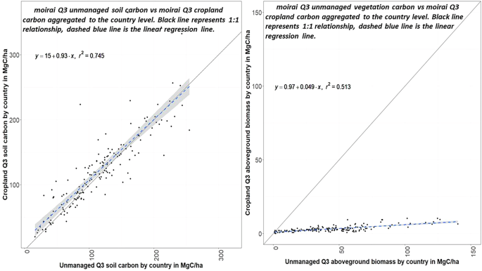
Comparison of unmanaged Q3 carbon stocks and Cropland carbon stocks for (A) soil carbon and (B) aboveground biomass. Values here are aggregated to individual countries.
In GCAM, crop yields are determined from harvested area and production data, while the carbon data are used for land use emissions and for valuing land carbon in global warming target scenarios. To address the relatively high cropland soil carbon data in our modeling experiments we reduce these data by 30% before using them in GCAM. Previous studies have found a similar loss of soil carbon through agricultural practices and land conver conversion from unmanaged land types to cropland38,39.
We performed a similar analysis for pasture carbon densities and found that pasture carbon shows depletion or lower values compared to unmanaged land cover both for both soil and vegetation. In this case, it is reasonable to use the Q3 soil and vegetation carbon values for pasture in GCAM without adjustment. This is an interesting case because pasture is not one of the source land types and its carbon values were assigned based on the same land types as for grassland. Multiple factors could contribute to this result, including sampling bias, pasture ___location bias, and uncertainties in data and processing. Nonetheless, these data capture the expected difference between pasture and unmanaged grassland.
-
Assesing spatial variability in soil and vegetation carbon within and across basins
We have established that carbon distributions within land regions generally follow a lognormal pattern for soil carbon and for vegetation carbon for most land types, except that forest vegetation carbon has a more bimodal distribution. However, there may be more dispersion across values in some basins for some land types compared to others. To assess this systematically, we computed a quartile coefficient of dispersion (QCD) for each basin and land type as:
$${{QCD}}_{{GLU},{LT},{pool}}={(Q3}_{{GLU},{LT},{pool}}-{Q1}_{{GLU},{LT},{pool}})/{(Q3}_{{GLU},{LT},{pool}}+{Q1}_{{GLU},{LT},{pool}})$$(5)Where,

pool is the carbon pool (aboveground biomass, belowground biomass, topsoil (0–30 cms)),
GLU represents a land region which is an intersection of basin boundaries and country boundaries,and LT is the land type.
The QCD values range from 0 to 1 where a value towards zero indicates less dispersion within a region-land type-carbon pool combination and a value towards 1 indicates more dispersion.
The QCD values for soil carbon (Fig. 11) are generally similar across most basins across land types. This is expected since the distributions of soil carbon are generally lognormal. However, in some basins the QCD value is consistently high and similar across land types. This mainly occurs in individual basins in Russia and Indonesia which have high levels of peat soils which would mean that the level of dispersion across cells would be high since some cells would contain peat soils whereaes others would not.

QCD values for topsoil carbon across basins and land types.
Based on QCD values across basins and land types for vegetation carbon (Fig. 12), we observe that there is significant variation in the QCD values within and across basins for tundra (with values ranging from 0-1). This is likely due to the way tundra pixels are defined in our dataset (they encompass different vegetation types). Similarly, there is significant variation within and across basins for grasslands, savannah and pastures, which is once again likely due to the definitions of what constitutes grasslands in the base land cover dataset. While there are also variations in vegetation carbon values for cropland and urban land, the overall range of values for these land types when it comes to vegetation carbon is low (Fig. 7). QCD values for forests across and between basins is lower. This may be due to the more narrow definitions for what constitutes forests across datasets.

QCD values for aboveground vegetation across basins and land type.
4E. Results from implementation of spatially explicit carbon in GCAM
As a final validation step, we separately implemented two carbon density sets from Moirai (3rd quartile, 90th percentile) and the Houghton densities in GCAM and compared these three cases. We make the following assumptions when implementing the carbon densities in GCAM, based on the analyses above:
-
Each set of carbon values are used throughout to reflect two potential options for a long-term potential maximum state of carbon in 1700
-
Cropland soil carbon is reduced by a factor of 0.3 (30% reduction) for all basins to reflect the effects of management. This is because we found that the soil carbon values do not show a depletion of carbon when comparing unmanaged soil carbon and crop carbon (See the findings of section 4D above)
-
Tundra, urban, desert, and polar desert/rock/ice do not change in GCAM and so the assigned carbon values do not influence model simulations. If a model does include dynamics for these land types, then the associated uncertainties should be addressed.
We emphasize that the results described here are GCAM specific and would be different based on the model selected.
4E (i) Results from historical spin up
We initialized GCAM using each of the three cases identified above. This resulted in a pre-spin up carbon stock of 1912 PgC (1320 PgC in soil and 591.7 PgC in vegetation) when using the Q3 state and a carbon stock of 2718 PgC (1753 PgC in top soil and 965 PgC in vegetation) when using the 90th percentile (Fig. 13 and Table 5). Note that these initialization values are calculated using the land cover in 1700, which does include some managed area, and the spatially explicit carbon. The same spin up values from Houghton et al. is 1905 PgC (1243 PgC in soil and 662 PgC in vegetation).

Descriptions of the results of the spin up process. Global vegetation carbon during spin up (1700–2015) and the SSP1 2p6 climate forcing scenario (2016–2100) for our initialization options.
During spin up this carbon is reduced to 1735 PgC in 2015 when using the Q3 state(1249 PgC of topsoil carbon and 486 PgC of vegetation carbon) as a result of historical land transitions (Fig. 13 and Table 5). Similarly during the spin up, this carbon is reduced to 2448 PgC when using the 90th percentile values (1655 PgC of topsoil carbon and 793 PgC of vegetation carbon). The same values from Houghton et al. is 1697 PgC (1181 PgC in soil and 516 PgC in vegetation).
An important point to note is that while the 90th percentile generates results more in line with independent pre-industrial estimates (Table 4), the Q3 state results in more realistic contemporary values in 2015 during the GCAM spin up (Figs. 8 and 9). For example, the Q3 state results in a contemporary value of 486 PgC of vegetation carbon in 2015, which is closer to contemporary vegetation carbon stock estimates. The Houhgton values produce a contemporary estimate of 516 PgC which is higher likely due to high estimates of tropical vegetation carbon.Whereaes, the 90th percentile results in a global vegetation carbon stock of 793 PgC. Using the 90th percentile would effectively result in an unrealistically high initial vegetation carbon stock that is close to equilibrium in 2015.
Another point to note is that the amount of global historical emissions (1700–2015) produced by the Q3 initialization is 176 PgC which is much lower than the global historial emissions using the 90th percentile of 270 PgC (Fig. 14). For context, the Global Carbon Project (as of 2021) produced an estimate of annual LUC emissions from 1700–2015 of 196 PgC40. The 90th percentile produces consistently higher annual LUC emissions than the other estimates, except for the dip in 2005. This dip is due to a shift in land use that accumulates excessive soil carbon rapidly in certain regions because of higher carbon densities in specific land types in the new spatially-explicit data.

Annual Global LUC emissions from GCP 2021 and our two initialization options.
Based on these spin up results and our validation analyses, we found that the Q3 value from our dataset is appropriate for initialization and use in GCAM when using the model to estimate contemporary C dynamics. While the 90th percentile better resembles independent estimates of pre-settlmenet stocks, it results in substantial overestimation when used to estimate contemporary C fluxes. This is a result of assumptions and processes within GCAM pertaining to carbon dynamics. Furthermore, the Q3 data provide a much less dramatic shift from the Houghton data previously used, than the 90th percentile data.
The appropriate carbon state for other models, which may implement carbon dynamics differently, could be different and would require a similar analysis. GCAM uses a simple bookkeeping approach to modeling carbon dynamics, with a primary assumption regarding the potential maximum carbon densitie of land types. The model begins by tracking a total stock of carbon for each water basin for each land type for two pools (soil and vegetation) in 1700. Following 1700 onwards, based on historical and future land use, the model calculates fluxes from this initial state. Sigmoidal growth curves are used to track regrowth of vegetation and exponential decay functions are used to track gain and loss in soil carbon. The model also calculates carbon fluxes based on net land use change (e.g. increase in cropland, reduction in forests) as opposed to gross transitions (e.g. cropland increase from grassland, cropland increase from forest loss).
4E (ii) Results from climate forcing scenario and sensitivity analysis
We use one climate forcing scenario with a maximum radiative forcing level of 2.6 watts per square meter by 2100 and shared socioeconomic pathway 1 (SSP1 2p6) to assess how the new carbon data influence land projection in GCAM. Under this scenario land carbon prices are implemented to assign value to terrestrial carbon at the same rate as carbon is valued in the energy system. SSP1 2p6 shows a large afforestation and more generally a large carbon response since it contains a carbon price while also having less stress from socio-economic factors across all IAMs41. GCAM by default uses carbon densities from Houghton et al.12, which are described in SI Table 2 (soil) and SI Table 3 (vegetation). Note that the changes in land cover under the climate forcing scenario are driven by relative levels of carbon across land types rather than absolute levels of carbon. Therefore, even if forest carbon in some tropical regions are lower than other estimates, forests still sequester much more carbon compared to other land types in these regions. We compare the same three cases as for the historical period: Houghton, the Moirai Q3 value, and the Moirai 90th percentile.
The global land allocation comparison under SSP1 2p6 scenario in GCAM (Fig. 15) shows that the afforestation/reforestation response is greatly reduced as a result of the spatially explicit carbon (the increase in forest cover from 2020 to 2100 globally is only 3.2 million km2 when using the moirai Q3 as opposed to 7 million km2 with the Houghton carbon). IAMs (Including GCAM) generally show a very optimistic afforestation response for this scenario that ranges from 0.5 to 12 million km2 of trees planted as part of a nature based carbon sequestration strategy under SSP1 2p641. The high afforestation response in some IAMs has been considered too optimistic by some studies (e.g.42). For Q3, the reduced forest expansion in GCAM with the new carbon data is largely driven by lower forest vegetation carbon densities in the new data, which reducd the incentive to expand forest. Conversely, the 90th percentile case reduces afforestation further, down to 0.1 million km2, even though the carbon densities are higher than for Q3. This is because smaller increases in forest cover are required to meet additional afforestation targets in the 90th percentile case. Despite the low afforestation, it adds another 54 PgC of vegetation carbon through afforestation that would result in an unrealistic value of vegetation carbon in 2100: about 847 PgC which is higher than undistrurbed carbon stocks in 1700. On the other hand, Q3 vegetation carbon stock in 2100 is close to 515 PgC (a dditional 30 PgC of carbon added through planted forests).Because the Q3 state reduces afforestation but maintains responsive land allocation and reasonable carbon accumulation, it is a better choice than the 90th percentile for initializing GCAM.

Global land allocation in GCAM under the SSP1 2p6 scenario by land type.
Global cropland and shrubland dynamics show a more complicated response than forest (Fig. 15). The reduced emphasis on forest expansion reduces the need for cropland abandonment. Cropland also sequesters more soil carbon in some regions (even with the 30% reduction factor), which also reduces abandonment. The shrubland response is also enhanced by higher shrubland vegetation carbon densities in the new spatially-explicit data.
Regional responses are dictated by their respective land type distrubutions. Generally, afforestion is maintained or enhanced in tropical forests and decreased in Boreal regions. For example, in Russia the afforestation strategy is completely replaced with a shrubland and grassland preservation strategy (SI Fig. 5). This is expected since the region has a relatively high amount of boreal forests. In South Asia however, where non-forest land types dominate, forest expansion persists and is supplemented by shrubland expansion (SI Fig. 6).
The implementation of the spatially explicit carbon clearly improves land use responses and also suggests that high carbon sequestering shrubs can also be preserved as a part of nature based solutions to mitigate climate change. The robustness of these responses across other radiative forcing scenarios (implemented for more SSPs for example) and across other models need to be studied and is a subject worthy of exploration in a future paper.
Usage Notes
In this paper we present a new dataset of grid-cell level, spatially-explicit carbon data harmonized with Moriai land data types. Our harmonized dataset presents carbon values for 3 pools (topsoil, above ground biomass and below ground biomass) for six statistical states for various land use types. Our dataset is available both at a 5 arcmin resolution and aggregated to 699 land regions. This dataset is designed to enable initialization of spatially explicit carbon in IAMs and MSD models, and we provide and example by applying it to GCAM. In the future, this dataset can be extended to include deeper soil (beyond 0–30 cms) so that land use responses in models can account for an additional deep soil carbon pool. We note however that if deeper soil carbon layers are to be added, regional and global models must also improve their respective carbon dynamics beyond simple bookkeeping approaches to include detailed accounting of environmental conditions.
We noted that there are some limitations with respect to the carbon observations (both for soil and vegetation) for tundra. For example, no data were found for 29% of the 5 arcmin gridcells for this land type. The biome mapping also needed to include several source land types to enable an increase in data coverage for tundra. This issue was likely caused by the different definitions of tundra land cover in different datasets. Recently, there have been efforts dedicated to collecting carbon data specifically for this land type. These data should be integrated in future releases of our data to address the current lack of data coverage.
As a part of our analysis, we observed that SoilGrids soil carbon values for cropland do not show a depletion when compared to SoilGrids soil carbon values in unmanaged land. As discussed, this is likely due the locations of sampling for cropland soil carbon. As a result, we reduced cropland soil carbon by 30% when we applied it to GCAM. This is in line with similar estimates of loss of soil carbon through agricultural practices and land conver conversion from unmanaged land types to cropland38,39. If better/improved data on crop soil carbon become available, our data could be updated with the same. Users should also consider % adjustments to crop soil carbon contents based on local cropping intensities.
We have also noted that our current estimates of forest vegetation carbon are based on both primary and secondary forests. This is due to the lack of availability of fine resolution (300 m) land masks that distinguish between primary and secondary forests. As more data become available related to forest cover types, a logical next step would be to break out different forest types in our dataset.
Finally, our analysis showed that using the Q3 statistical state was most appropriate for GCAM even though it resulted in an initialization of pre-industrial carbon value that was lower than other estimates. Selection of the Q3 results in more accurate historical LUC emissions and the model therefore spins up to a value that is close to other estimates in the literature in 2015.
The data are derived for several statistical states (with the Q3 being one of them) for a data-derived set of land types that are not model specific. The resulting dataset is then applied to GCAM as an example. This example for GCAM shows how we analyzed the data to select the appropriate value for GCAM, which includes analysis of the statistical range of options across the spatial distribution. Specific data uncertainty analyses have already been performed on the source data by their creators. Like any dataset, a user must determine how to use it for their particular application and model, and perform the required processing.
While we use the data from 2010, we emphasize once more that we utilize contemporary data to extract statistical states to select a potential carbon value that can be used for calibrating the model. More specifically our q3 value selected from the 2010 values is used as a potential carbon density that a model builds towards and is used to spin up the model as seen in our results. We also note that the year 2010 is selected since the SoilGrids and Spawn et al. data are based on land masks for that year. The usage of more contemporary data may not affect this analysis in any significant way (unless the overall distribution of carbon is altered).
Code availability
As mentioned above, the data can be generated programmatically with scripts that are hosted on GitHub (https://github.com/JGCRI/moirai/tree/master/ancillary/carbon_harmonization). The process has been split into two steps where the computationally intensive stage 1 (approx.. 6 hours of processing) is optional with outputs made available in the repository. The Stage 1 processing is performed using bash scripts which use the GDAL software36. The second stage processing uses an R script and can be completed for all carbon pools in approx. 15 minutes to generate the final 72 rasters and the final tabular output file. We have also made available optional diagnostic functions in the R script which can be used to validate results.
References
Calvin, K. et al. GCAM v5. 1: representing the linkages between energy, water, land, climate, and economic systems. Geoscientific Model Development 12(2), 677–698 (2019).
Binsted, M. et al. GCAM-USA v5.3_water_dispatch: integrated modeling of subnational US energy, water, and land systems within a global framework. Geoscientific Model Development Discussions 1–39 (2021).
Calvin, K. V. & Bond-Lamberty, B. P. Integrated human-earth system modeling. In AGU Fall Meeting Abstracts. 2018, pp. U14A-02. (2018).
Thomson, A. M. et al. Climate mitigation and the future of tropical landscapes. Proceedings of the National Academy of Sciences 107(46), 19633–19638 (2010).
Wise, M. et al. Implications of limiting CO2 concentrations for land use and energy. Science 324(5931), 1183–1186 (2009).
Gibbs, H., Yui, S. & Plevin, R. J. New estimates of soil and biomass carbon stocks for global economic models (2014).
Angel, A., Maksym, C., Corong, E. & van der Mensbrugghe, D. The global trade analysis project (GTAP) data base: Version 11. Journal of Global Economic Analysis 7(2) (2022).
Frank, S. et al. Documentation for estimating LULUCF emissions/removals and mitigation potentials with GLOBIOM/G4M. https://climate.ec.europa.eu/system/files/2021-08/lulucf_methodology_report_en.pdf (2020).
Erb, K.-H. et al. Unexpectedly large impact of forest management and grazing on global vegetation biomass. Nature 553(7686), 73–76 (2018).
Walker, W. S. et al. The global potential for increased storage of carbon on land. Proceedings of the National Academy of Sciences 119(23), e2111312119 (2022).
Fang, Y., Liu, C., Huang, M., Li, H. & Leung, L. R. Steady state estimation of soil organic carbon using satellite‐derived canopy leaf area index. Journal of Advances in Modeling Earth Systems 6(4), 1049–1064 (2014).
Houghton, R. A. The annual net flux of carbon to the atmosphere from changes in land use 1850–1990. Tellus B 51(2), 298–313 (1999).
Jackson, R. B. et al. The ecology of soil carbon: pools, vulnerabilities, and biotic and abiotic controls. Annual Review of Ecology, Evolution, and Systematics 48(1), 419–445 (2017).
Nachtergaele, F., et al The harmonized world soil database. Proceedings of the 19th World Congress of Soil Science, Soil Solutions for a Changing World, Brisbane, Australia, 1-6 August 2010 (2010).
Batjes, N. H. et al. WoSIS: providing standardised soil profile data for the world. Earth System Science Data 9(1), 1–14 (2017).
Hengl, T. et al. SoilGrids1km—global soil information based on automated mapping. PloS one 9(8), e105992 (2014).
Jungkunst, H. F., Göpel, J., Horvath, T., Ott, S., & Brunn, M. Global soil organic carbon–climate interactions: Why scales matter. Wiley Interdisciplinary Reviews: Climate Change, e780 (2022).
Li, W. et al. Gross and net land cover changes in the main plant functional types derived from the annual ESA CCI land cover maps (1992–2015). Earth System Science Data 10(1), 219–234 (2018).
Liu, X. et al. Identifying patterns and hotspots of global land cover transitions using the ESA CCI Land Cover dataset. Remote Sensing Letters 9(10), 972–981 (2018).
Klein Goldewijk, K., Beusen, A., Doelman, J. & Stehfest, E. Anthropogenic land use estimates for the Holocene–HYDE 3.2. Earth System Science Data 9(2), 927–953 (2017).
Barnes, W. L., Xiong, X. & Salomonson, V. V. Status of terra MODIS and aqua MODIS. Advances in Space Research 32(11), 2099–2106 (2003).
Justice, C. et al. An overview of MODIS Land data processing and product status. Remote sensing of Environment 83(1-2), 3–15 (2002).
van Asselen, S. & Verburg, P. H. AL and System representation for global assessments and land‐use modeling. Global Change Biology 18(10), 3125–3148 (2012).
Spawn, S. A., Sullivan, C. C., Lark, T. J. & Gibbs, H. K. Harmonized global maps of above and belowground biomass carbon density in the year 2010. Scientific Data 7(1), 1–22. (2020).
Di Vittorio, A. V., Vernon, C. R., & Shu, S. Moirai version 3: a data processing system to generate recent historical land inputs for global modeling applications at various scales. Journal of Open Research Software, 8(PNNL-SA-142149) (2020).
Sanderman, J., Hengl, T. & Fiske, G. J. Soil carbon debt of 12,000 years of human land use. Proceedings of the National Academy of Sciences 114(36), 9575–9580 (2017).
Scharlemann, J. P., Tanner, E. V., Hiederer, R. & Kapos, V. Global soil carbon: understanding and managing the largest terrestrial carbon pool. Carbon Management 5(1), 81–91 (2014).
Tifafi, M., Guenet, B. & Hatté, C. Large differences in global and regional total soil carbon stock estimates based on SoilGrids, HWSD, and NCSCD: Intercomparison and evaluation based on field data from USA, England, Wales, and France. Global Biogeochemical Cycles 32(1), 42–56 (2018).
Warmerdam, F. Open source approaches in spatial data handling. by Hall, GB & Leahy, MG Berlin, Heidelberg: Springer Berlin Heidelberg, 87-104 (2008).
Meiyappan, P. & Jain, A. K. Three distinct global estimates of historical land-cover change and land-use conversions for over 200 years. Frontiers of earth science 6(2), 122–139 (2012).
Ramankutty, N. & Foley, J. A. Estimating historical changes in land cover: North American croplands from 1850 to 1992: GCTE/LUCC RESEARCH ARTICLE. Global Ecology and Biogeography 8(5), 381–396 (1999).
Hugelius, G. et al. Estimated stocks of circumpolar permafrost carbon with quantified uncertainty ranges and identified data gaps. Biogeosciences 11(23), 6573–6593 (2014).
Tesfa, T. K. et al. Scalability of grid- and subbasin-based land surface modeling approaches for hydrologic simulations. Journal of Geophysical Research: Atmospheres 119(6), 3166-3184 (2014).
Narayan, K. B., Di Vittorio, A. V., Margiotta, E., Spawn, S. A. & Gibbs, H. A. Spatially explicit re-harmonized terrestrial carbon stocks for calibrating Integrated Multisectoral Models (v2) [Data set]. Zenodo https://doi.org/10.5281/zenodo.13988220 (2024).
Vlek, P. L., Khamzina, A. & Tamene, L. Land degradation and the Sustainable Development Goals. (2017).
Poggio, L. et al. SoilGrids 2.0: producing soil information for the globe with quantified spatial uncertainty. Soil 7(1), 217–240 (2021).
Houghton, R. Aboveground forest biomass and the global carbon balance. Global Change Biology 11(6), 945–958 (2005).
Cooper, H., Sjögersten, S., Lark, R. & Mooney, S. To till or not to till in a temperate ecosystem? Implications for climate change mitigation. Environmental Research Letters 16(5), 054022 (2021).
Wei, X., Shao, M., Gale, W. & Li, L. Global pattern of soil carbon losses due to the conversion of forests to agricultural land. Scientific reports 4(1), 1–6 (2014).
Friedlingstein, P. et al. Global carbon budget 2021. Earth System Science Data 14(4), 1917–2005 (2022).
Popp, A. et al. Land-use futures in the shared socio-economic pathways. Global Environmental Change 42, 331–345 (2017).
Pongratz, J. et al Land use effects on climate: current state, recent progress, and emerging topics. Current Climate Change Reports, 1-22 (2021).
Acknowledgements
This research was supported by the U.S. Department of Energy, Office of Science, as part of research in Multi Sector Dynamics, Earth and Environmental System Modeling Program. The Pacific Northwest National Laboratory is operated for DOE by Battelle Memorial Institute under contract DE-AC05-76RL01830
Author information
Authors and Affiliations
Contributions
K.B.N., A.D.V. conceived the concept of this paper. K.B.N., A.D.V. and E.V. produced the data from the raw input files and also made code changes to the moirai land data system. S.S.L. and H.G. produced the vegetation carbon data required by this study and also provided inputs on data interpretation. K.B.N., A.D.V. wrote the manuscript with input from all authors.
Corresponding author
Ethics declarations
Competing interests
The authors declare no competing interests.
Additional information
Publisher’s note Springer Nature remains neutral with regard to jurisdictional claims in published maps and institutional affiliations.
Supplementary information
41597_2025_4723_MOESM1_ESM.docx
Supplementary information for “Spatially explicit re-harmonized terrestrial carbon densities for calibrating Integrated Multisectoral Models
Rights and permissions
Open Access This article is licensed under a Creative Commons Attribution-NonCommercial-NoDerivatives 4.0 International License, which permits any non-commercial use, sharing, distribution and reproduction in any medium or format, as long as you give appropriate credit to the original author(s) and the source, provide a link to the Creative Commons licence, and indicate if you modified the licensed material. You do not have permission under this licence to share adapted material derived from this article or parts of it. The images or other third party material in this article are included in the article’s Creative Commons licence, unless indicated otherwise in a credit line to the material. If material is not included in the article’s Creative Commons licence and your intended use is not permitted by statutory regulation or exceeds the permitted use, you will need to obtain permission directly from the copyright holder. To view a copy of this licence, visit http://creativecommons.org/licenses/by-nc-nd/4.0/.
About this article

Cite this article
Narayan, K.B., Di Vittorio, A.V., Margiotta, E. et al. Spatially explicit terrestrial carbon densities for calibrating the carbon cycle in human-Earth system Models. Sci Data 12, 638 (2025). https://doi.org/10.1038/s41597-025-04723-4
Received:
Accepted:
Published:
DOI: https://doi.org/10.1038/s41597-025-04723-4
