
Abstract
Paleoclimate model simulations provide reference data to help interpret the geological record and offer a unique opportunity to evaluate the performance of current models under diverse boundary conditions. Here, we present a dataset of 35 climate model simulations of the warm early Eocene Climatic Optimum (EECO; ~ 50 million years ago) and corresponding preindustrial reference experiments. To streamline the use of the data, we apply standardised naming conventions and quality checks across eight modelling groups that have carried out coordinated simulations as part of the Deep-Time Model Intercomparison Project (DeepMIP). Gridded model fields can be downloaded from an online repository or accessed through a new web application that provides interactive data exploration. Local model data can be extracted in CSV format or visualised online for streamlined model-data comparisons. Additionally, processing and visualisation code templates may serve as a starting point for advanced analysis. The dataset and online platform aim to simplify accessing and handling complex data, prevent common processing issues, and facilitate the sharing of climate model data across disciplines.
Background & Summary
Past climate changes provide an opportunity to better understand how key components of the climate system might change under anthropogenic greenhouse gas emissions and thus help constrain future climate change1. Comparisons with paleoclimate data allow us to evaluate climate models under atmospheric CO2 scenarios similar to those possible in the near future. Furthermore, these paleoclimate model simulations provide global, physically consistent reference data to support the interpretation of paleoclimatic data across a wide range of disciplines, e.g. in geology, biology, and geochemistry.
One of the most well-studied deep-time intervals with respect to model-data comparison is the early Eocene Climatic Optimum (EECO; ~53.3 to 49.1 million years ago2) as it provides an analogue for future very high emission scenarios3. It was characterised by atmospheric CO2 concentrations of ~1,500 ppmv4 and global mean surface temperatures (GMSTs) 10 to 16°C warmer than pre-industrial5. Several modelling studies have focused on improving our understanding of the mechanisms and implications of EECO warmth6,7,8,9,10 and ultimately motivated the formulation of the Eocene Modelling Intercomparison Project (EoMIP)11. While limited due to its opportunistic design, EoMIP nonetheless highlighted the possibility of using multi-model ensembles to systematically assess model-model and model-data differences in our understanding of Eocene climate.
Building on this potential, DeepMIP - the Deep-Time Model Intercomparison Project - was designed to provide a consistent framework to carry out coordinated EECO model experiments12. Eight modelling groups performed a total of 35 model simulations using the same paleogeographic and vegetation boundary conditions at a range of atmospheric CO2 concentrations (Table 1). These new simulations showed more consistent global mean surface temperatures across the ensemble and larger climate sensitivities compared to the EoMIP results13. The coordinated experiment set-up allowed a separation of the relative influence of changes in CO2 concentrations and non-CO2 boundary conditions (i.e. removal of land ice and prescribed vegetation) on the simulated surface temperatures. Non-CO2 boundary conditions alone lead to 3-5°C overall warming and contribute substantially to the reduced meridional temperature gradient, while higher CO2 levels drive global mean warming due to decreases in atmospheric emissivity. Importantly, three models (CESM1.2-CAM5, GFDL-CM2.1 and NorESM1-F) were able to produce absolute GMSTs and reduced meridional temperature gradients consistent with the geological record at CO2 concentrations within the reported range of EECO reconstructions (1170 to 2490 ppmv14).
The DeepMIP-Eocene ensemble has already been used in multiple studies, analysing specific aspects of the Eocene climate in more detail, e.g. the meridional temperature gradient15, the surface to deep ocean temperature relationship16, ocean circulation17, sea ice18, hydroclimate19,20,21,22,23, and the impact of mountains24,25. We anticipate continued interest in the DeepMIP-Eocene model data, both for model intercomparisons and for model-data syntheses, and aim to document the design of the dataset and streamline access to improve future reuse of the data. Although the use of large model ensembles is helpful in quantifying the influence of uncertainties in boundary conditions and limitations in model performance on the simulated Eocene climate, it also presents a technical hurdle in accessing and fully utilising the available data. The use of model-specific data standards, post-processing workflows and variable naming schemes can make the analysis and comparison of multi-model ensembles a tedious process or even lead to processing errors. The need for significant data processing expertise can therefore limit the benefits and wider use of these important data, particularly in non-modelling paleoclimatology disciplines.
Here, we build on the DeepMIP framework to address these issues and present standardised, quality-checked EECO model output to facilitate multi-model processing and analysis, both for model intercomparisons and model-data comparisons. We have reprocessed the output of a total of 26 EECO simulations at CO2 concentrations between ×1 and ×9 pre-industrial levels, together with their nine pre-industrial reference experiments, to generate a dataset of common climate variables with consistent temporal averaging, variable names and units across the ensemble. We follow the CMIP convention for variable names and units as closely as possible to take advantage of existing processing workflows, and use the ensemble spread to quantify the internal consistency of the output fields.
We provide two complementary ways of accessing the dataset, tailored to the most likely future use cases. First, the entire dataset is stored as global, gridded netCDF (network Common Data Form) files in the Centre for Environmental Data Analysis (CEDA) Archive and can be downloaded as individual files or in batch mode26. Combined with the consistent DeepMIP naming convention, this provides a more traditional, scriptable starting point for further analysis. This approach shares the goals of other existing infrastructure projects for sharing climate model data such as the Earth System Grid Federation (ESGF)27, but the limited scope and overall much smaller file sizes of this dataset allow us to use centralised, rather than distributed, data storage for greater user convenience. Second, we present an interactive web application to facilitate model-data comparisons of EECO surface temperatures and precipitation. This is a very common use case for paleoclimate model data, but also involves multiple processing steps and potential pitfalls, especially when working with a large model ensemble. Modern web technologies provide the opportunity for intuitive, browser-based access to complex data and, therefore, the possibility to assist users in extracting subsets of relevant information for them. Recent examples include the Interactive Atlas28 of the Intergovernmental Panel on Climate Change (https://interactive-atlas.ipcc.ch, last access: 26 June 2024) and the Copernicus Interactive Climate Atlas created by the Copernicus Climate Change Service (https://atlas.climate.copernicus.eu/atlas, last access: 26 June 2024). The DeepMIP web application follows a similar approach by providing intuitive data access and custom workflows to simplify common model-data comparison tasks. The web application automatically calculates paleolocations for a single site or a list of present-day locations, extracts the corresponding model data from the various model grids and plots a summary of the results. The resulting data can be exported for further offline analysis, while the underlying Python code can be used as a starting point for custom analysis.
The dataset and tools provided are designed to enable data access for non-programmers and to streamline analysis for more advanced users to routinely evaluate existing and emerging paleoclimate data against the full DeepMIP-Eocene model ensemble. This will help to bridge the gap between modelling and data communities to ultimately advance our understanding of early Eocene climate and could potentially serve as a reference framework for similar projects of other geological time periods in the future.
Methods
DeepMIP-Eocene experiments
All EECO simulations that follow the DeepMIP-Eocene experimental design protocol12 and were completed by September 2023 form the input data for version 1.0 of the dataset (Table 1). These simulations are identical to those described in the DeepMIP overview paper13, with the exception of the new MIROC ×1 and ×2 experiments. The DeepMIP framework provides standardised model boundary conditions and experimental designs to allow a coordinated model intercomparison of the simulation results. All groups have used one of the two reference paleogeographic reconstructions29,30 (Fig. 1a-b) interpolated to their respective model grids. The main difference between the two available paleogeographies is the choice of the applied rotation reference frame leading to slight differences in the relative positions of individual plates (Fig. 1c). Prescribed vegetation and river runoff follow a published reconstruction29, while globally homogeneous soil parameters based on the global mean of the respective pre-industrial simulation were used. All groups provided a pre-industrial reference simulation and performed a series of EECO experiments, differing only in the concentration of atmospheric CO2, summarised in Table 2. Other greenhouse gas concentrations and the solar constant were held constant at their pre-industrial levels.

A complete overview of the modelling framework is given in the DeepMIP experimental design paper12, and detailed descriptions of its implementation in the individual models can be found in the analysis of the large-scale climatic features13. We also provide a full description of each model setup based on their published method sections13 as a README file in the dataset itself. This is intended to make the downloaded files self-describing and to allow dynamic addition of new experiments and models in the future. In the following, for each model included in version 1.0 of the dataset, we provide a brief summary of the initialisation and spin-up strategies, as this step required individual decisions by each modelling group. The DeepMIP experimental design provides an idealised equation for initialising the ocean temperatures as:
where ϕ is latitude, and z is ocean depth. The parameters A, B and D are specified in the experimental design as 25, 15 and 5000, respectively12. The resulting warm ocean temperatures caused numerical problems in some model spin-ups and have therefore been modified for individual models. An overview of the parameters used for each model is given in Table 3. Any other deviations for the model initialisation are listed below.
CESM
Ocean temperatures and salinities in all Eocene simulations are initialised from the same Palaeocene-Eocene Thermal Maximum (PETM; ~55 million years ago) experiment using a previous version of CESM31,32. The ×1 simulation was integrated for a further 2600 years, while all other experiments were run for 2000 years. The mean top of the atmosphere (TOA) imbalance over the last 100 model years for the PI, ×1, ×3, ×6 and ×9 experiments are −0.05, −0.25, −0.32, 0.34 and 0.64 Wm−2, respectively.
COSMOS
The ×3 integration was initialised with a homogeneous temperature and salinity of 10°C and 34.7 psu, respectively, and integrated for an initial 1000 years, after which the ×1 and ×4 simulations were branched. After an initial 8000 years with transient orbital parameters, a constant, pre-industrial orbital configuration was used for the final 1500 years of all simulations. Instead of using the proposed river routing scheme29, the simulations use a hydrological discharge model that follows the model orography33. The mean TOA imbalance over the last 100 model years for the PI, ×1, ×3 and ×4 experiments are 1.75, 1.91, 1.78, and 1.95 Wm−2, respectively.
GFDL
The ×1, ×2, ×3, and ×4 simulations were started with a globally homogeneous salinity of 34.7 psu and a slightly cooler version of the DeepMIP temperature equation (Eq. (1); Table 3). After 1500 and 2000 years of integration, an acceleration technique was applied. Specifically, the linear temperature trends of the last 100 years for each model level below 500 m were calculated and the level-by-level temperatures were then extrapolated by 1000 years following this trend. After the second application of this technique at year 2000, the model was run out normally for a further 4000 years for a total of 6000 years. The ×6 simulation was initialised with a globally uniform temperature of 19.32°C and continously integrated for 6000 years. The mean TOA imbalance over the last 100 model years for the PI, ×1, ×2, ×3, ×4 and ×6 experiments are 0.31, 0.10, −0.08, −0.14, −0.19, and −0.28 Wm−2, respectively.
HadCM3
Initial ocean temperatures for HadCM3BL were derived from an idealised temperature profile with lowered, CO2 dependent deep ocean temperatures based on previous Eocene simulations. HadCM3B experiments were branched from the respective HadCM3BL simulations after 4400 to 4900 years and integrated for a further 2950 years. Multiple ocean gateways in the original paleogeography were widened to allow unrestricted ocean circulation and to guarantee the same gateway widths on both the low and high-resolution ocean grids of HadCM3BL and HadCM3B, respectively. In addition, maximum water depths in parts of the Arctic Ocean were reduced to improve numerical stability. The mean TOA imbalance per century averaged over the last 50 model years for the PI, ×1, ×2 and ×3 experiments for HadCM3B are −0.08, −0.02, −0.08 and −0.08 Wm−2, respectively.
INMCM
The ocean temperature and salinity in the ×6 simulation follow the idealised equations of the DeepMIP protocol, but with equatorial surface temperatures lowered by 5°C (Eq. (1); Table 3). The simulation was integrated for a total of 1150 years. The mean TOA imbalance over the last 100 model years for the PI and ×6 experiments are 4.37 and 2.87 Wm−2, respectively.
IPSL
A modified version of Eq. (1) with overall reduced subsurface temperatures (Table 3) and a globally homogeneous salinity of 34.7 psu were used to initialise the ×3 simulation. The ×1.5 simulation is branched from the ×3 experiment after 1500 years. Both simulations are run for a total of 4000 years. The ocean bathymetry around individual ocean straits has been manually adjusted to guarantee the minimum gateway width necessary to allow throughflow. The mean TOA imbalance over the last 100 model years for the PI, ×1.5 and ×3 experiments are 0.08, 0.59 and 0.76 Wm−2, respectively.
MIROC
All three simulations have been initialised with a modified version of the idealised DeepMIP temperature equation, with ocean temperatures globally reduced by 15°C (Eq. (1); Table 3), and integrated for 5000 model years. The ×1 and ×2 experiments are new and have not been included in the DeepMIP overview paper13. The mean TOA imbalance over the last 100 model years for the PI, ×1, ×2 and ×3 experiments are 0.96, 0.79, 0.91 and 0.96 Wm−2, respectively.
NorESM
Initial ocean temperatures for the ×2 simulation were used from a previous NorESM-L simulation34, while salinities were set to 25.5 psu in the Arctic and 34.5 elsewhere. The ×4 simulation was branched off after 100 model years, and both simulations have been run for a further 2000 years. The NorESM simulations were performed with a different paleogeographic reconstruction than the rest of the DeepMIP ensemble (Table 1). The mean TOA imbalance per century at the end of the PI, ×2 and ×4 experiments are −0.02, 0.03 and 0.24 Wm−2, respectively. Note that the PI imbalance is calculated over the last 1000 years, while the Eocene values are averaged over the last 100 years.
Data processing
We use the raw output of the last 100 years of each of the 35 model simulations as input for our post-processing. For each variable, we generate up to three netCDF output files to facilitate common analysis workflows. We always produce a mean file representing either the monthly mean climatology or the annual mean averaged over the last 100 model years, depending on the temporal resolution of the model output. In case of monthly mean output data, the std file contains the standard deviation over the same averaging period for each month of the year and can be used for significance testing. Where feasible, we also store the full monthly mean output of the last 100 model years as a time_series file to investigate temporal trends or interannual variability.
Alongside this standard output, we provide a generic script to interpolate model fields from their native grids to a common resolution for model intercomparisons. The processing workflow requires a local installation of the Climate Data Operator (CDO) software35 for bilinear or nearest-neighbour interpolation for atmosphere and ocean variables, respectively. The processing script is distributed as part of the dataset (see Data Records section).
Naming convention
We employ a consistent naming convention for variables, directories, and file names across all models to simplify the comparison of different models and to allow a scripted analysis of the entire dataset. The list of output variables is an extended version of those proposed in the DeepMIP experimental design12 and is shown in Tables 4-5. Variable names, units and signs of fluxes follow the naming convention of the Coupled Model Intercomparison Project 6 (CMIP6) data request (https://wcrp-cmip.github.io/WGCM_Infrastructure_Panel/CMIP6/data_request.html, last access: 26 June 2024). Consistent standard names, long names and global attributes are directly added to the netCDF files following the Climate and Forecast metadata conventions (CF36) in version 1.8 (http://cfconventions.org, last access: 26 June 2024). All netCDF file have been automatically tested for CF-compliance with the cf-checker utility (https://github.com/cedadev/cf-checker, last access: 26 June 2024) developed by the UK Met Office and the NCAS Computational Modelling Services (NCAS-CMS). Following the CMIP and CF community standards will both increase user familiarity with the new dataset and will allow the integration into existing analysis workflows and software. Each output variable is stored in a separate file according to the following structure:
directory = deepmip-eocene-p1/<Family>/<Model>/<Experiment>/<Version>/<Averaging>/
filename = <Variable>_<Model>_<Experiment>_<Version>.<Statistic>.nc
-
<Family>, <Model> and <Experiment> are listed in Tables 1 and 2, respectively
-
<Variable> represents the first column in Tables 4-5
Table 5 Ocean output variables included in version 1.0 of the dataset. Naming conventions follow the CMIP6 data request. -
<Statistic> is either mean (1 or 12 timsteps), std (12 timsteps), time_series (1200 timsteps) or omitted for the time-independent boundary conditions
-
the smaller mean and std files are stored in the <Averaging>=climatology directory and are separated from the larger time_series files in the <Averaging>=time_series directory to enable more granular download options
Storing all relevant information in the file name itself also allows new phases of coordinated DeepMIP simulations to be integrated into a single dataset in the future.
Data Records
The full dataset has been deposited in the CEDA Archive, the UK national data centre for atmospheric and earth observation research26. This dataset contains the following types of files:
-
model data: The directory deepmip-eocene-p1 contains all processed model output in CF compliant netCDF format37, a self-describing community standard for storing gridded simulation data, with a total file size of 168.0 GB. Directory and file structure follow the DeepMIP naming convention described above.
-
model READMEs: Each <Family> top-level directory contains a single <Family>_README.md file that contains detailed information about the model, the simulation setup, and naming convention. This ensures the downloaded dataset is sufficiently self-described and allows the addition of new models and simulation results in the future.
In addition, the code of the web application38 and a collection of scripts and metadata to interact with the dataset39 are deposited in separate Zenodo repositories. The latter includes a collection of Python code to interpolate model data to a common grid (regrid_deepmip_data.py), recreate the validation tables of available data (plot_z-scores.py) and Python dictionaries containing available DeepMIP models, experiments and variables to support scripted analysis of the dataset.
Technical Validation
An earlier version of the dataset has already been used in a number of publications13,15,16,18,19,20,21,24,25 to assess the scientific validity of the model simulations, both in terms of model-model and model-data comparisons. In this section, we verify the internal consistency of the dataset, ensuring that the naming convention has been applied correctly and that the resulting variable names, units and fluxes are consistent across all models. To do this, we automatically parse all mean and time_series files in the dataset for any given experiment, interpolate them to a common grid, calculate the global mean, minimum and maximum values and compare these values across all models. We use annual mean fields for the validation of mean files and the last 12 available months of the time_series files. For variables with multiple vertical levels (see Tables 4-5), we select the vertical index nearest to the 500 hPa pressure level or 1000 m depth for atmospheric and ocean data, respectively. Example tables for atmospheric and ocean mean variables from the ×3 simulations are shown in Figs. 2 and 3, tables for all other experiments as well as for time_series files are uploaded to the web application. This testing procedure simulates a standard analysis workflow and is able to detect any deviations from the expected DeepMIP naming convention, while the resulting tables provide a visual overview of the available model fields for each experiment. We further calculate the median and standard deviation for each variable and metric across all available models (i.e. for each row in the table) to flag potential outliers that may arise due to inconsistent units or different directions of energy or mass fluxes. For this, we calculate a z-score for each model, variable and statistic which quantifies the number of standard deviations an individual model statistic is above or below the ensemble median. We use the ensemble median instead of the mean as the reference point to reduce the influence of potential outliers in our small sample sizes and calculate the adjusted z-scores as:
where z is the computed z-score, x is the individual model value, M is the median across all available models for the respective variable and statistic (i.e., across each table row), and σ is the standard deviation across the ensemble. A z-score > 3 is commonly used as a cut-off to identify outliers in a distribution. Due to the small sample sizes (N ≤ 9) the z-score threshold was not used to exclude any data from the dataset, but rather to find and resolve inconsistencies in the data processing between the models. For this, the background of each cell in Figs. 2 and 3 has been coloured by their computed z-score to visually identify model results substantially different from the ensemble median. Note that all modelling groups have performed slightly different sets of simulations (Table 1) and not all models provide all requested output variables. These fields are indicated by gray “nan” cells in the overviw tables. For example, INM and NorESM did not perform a ×3 experiment and are therfore not included in Fig. 2 and Fig. 3. In the final dataset, all available model fields are within ±3 standard deviations around the respective ensemble median, although we note that the small sample sizes allow only an indicative analysis. The Python processing code is included in the online dataset (see Data Records section) and can be used to develop a custom analysis workflow or to validate any regridding and global averaging performed by the user.

Technical validation of atmospheric global model fields of the ×3 experiment across the ensemble. Variables with multiple vertical levels are shown for the respective model pressure level closest to 500 hPa. Tables for other experiments and “time_series” files can be found in the web application at https://data.deepmip.org/Validation_tables. Note that the INM and NorESM models did not perform the ×3 experiment (Table 1) and are therefore excluded from this analysis.

Technical validation of ocean global model fields of the ×3 experiment across the ensemble. Variables with multiple vertical levels are shown for the respective model depth closest to 1000 m. Tables for other experiments and “time_series” files can be found in the web application at https://data.deepmip.org/Validation_tables. Note that the INM and NorESM models did not perform the ×3 experiment (Table 1) and are therefore excluded from this analysis.
Usage Notes
We present two primary routes to access the dataset, either via downloading the netCDF files for local processing or via an interactive website for online model-data comparisons.
netCDF repository
First, processed netCDF files for all simulations are available from the CEDA Archive26. The full directory structure can be accessed via the browser and files can be downloaded via HTTP, Wget, FTP or OPeNDAP. This allows easy access to the data via the browser, as well as scriptable interfaces for bulk downloading. The OPeNDAP (Open-source Project for a Network Data Access Protocol) protocol allows the remote subsetting and exploration of datasets directly in e.g. Python, R, IDL, and Matlab. The CEDA Archive website (https://help.ceda.ac.uk/article/99-download-data-from-ceda-archives; last access: 26 June 2024) provides an up-to-date overview of all available access options.
Interactive web application
Second, simulated surface temperatures and precipitation from any ___location can be extracted, visualised and downloaded at https://data.deepmip.org. This allows model-data comparisons via a simple user interface without the need to download the netCDF files locally. The website is designed to extract surface temperature and precipitation for any user-defined ___location from all available model simulations and either visualise the results or download them for offline use. All processing code is written in Python and bundled into a web application via the Streamlit library (https://streamlit.io; last access: 26 June 2024). The code makes full use of the naming conventions described above and is therefore general enough to serve as a template for further in-depth analysis. The sidebar of the web application can be used to choose between three different analysis pages:
-
1.
Extract local model data: Finds the model data closest to a user-specified site (see example in Fig. 4). The minimum inputs are the modern ___location of the site and the variable of interest (either near-surface air temperature, sea surface temperature, or total precipitation). The application will automatically reconstruct the site’s EECO paleo-position on both the mantle29 and paleomagnetic30 reference frames and extract the respective monthly and annual mean simulation data from the closest grid point for all models in the dataset. Model data is interpolated to a common 1° × 1° grid (see Data processing section for details) prior to the data selection to eliminate the influence of different model resolutions on the results. In the end, the ensemble means for each experiment are calculated and the results are listed in an interactive table. Data can be downloaded in CSV, Excel or JSON format for direct import into spreadsheets for further offline analysis. The extraction can be performed for a single site or a list of locations and all sites from the DeepMIP proxy dataset2 are pre-loaded and available for comparison with the simulation results. Furthermore, the underlying Python functions get_paleo_locations() and get_model_point_data() are available in the deepmip_modules.py file of the application repository for reuse in any custom analysis. The get_paleo_locations() function uses the paleolocation lookup fields provided in the experimental design paper12 to find the respective early Eocene locations for a list of modern latitude/longitude pairs, using both the mantle29 and paleomagnetic30 reference frames. Results are saved in a Pandas DataFrame which can be directly passed to get_model_point_data() to extract the nearest model data for all reconstructed locations.
Fig. 4 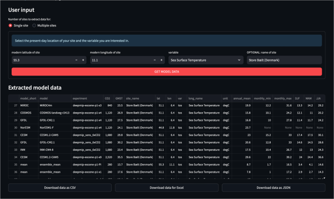
Example user input and extracted model data for a single site in the web application.
-
2.
Plot local model data: Visualises the extracted results and optionally compares them to proxy reconstructions (see example in Fig. 5). Available visualisations include line plots of the annual cycle at the user-specified ___location, grouped by the various DeepMIP CO2 levels (Fig. 5a), and a scatter plot of all simulated annual mean values against the respective GMSTs or CO2 concentrations of the model simulations. (Fig. 5b). The latter plot type can be useful to compare the sensitivity of the model results at the local site against global climate signals. The simulated monthly and annual mean model results can be visually compared against a local proxy reconstruction, either by manually specifying the mean and standard deviation of the proxy data or by loading the respective values for locations from the DeepMIP proxy dataset2. The user can zoom and pan within the interactive figures and download them in PNG and SVG format.
Fig. 5 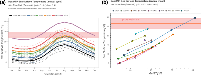
Example graphical output of the web application for the model-data comparison of the Store Bælt (Denmark) site defined in Fig. 4. (a) Simulated annual cycle of sea surface temperatures at the respective grid point closest to the reconstructed paleoposition of the site. Solid lines show the ensemble mean for each CO2 concentration with individual models represented by the dashed lines. (b) Scatter plot of the simulated annual mean sea surface temperature at the proxy site compared to the global mean surface temperature of the respective simulation. Lines connect results of the same model. Reconstructed proxy temperature is based on the TEX86 paleothermometer2.
-
3.
Map sites and boundary conditions: Plots paleogeographic maps of the chosen site. The user can choose between a global map indicating the ___location of the study site or regional maps of the bathymetry, orography and land-sea mask on the various native model grids (Fig. 6). The latter can help with the interpretation of the model-data comparison result, e.g. by visualising local grid resolutions and associated intermodel differences in the representation of mountain ranges or ocean gateways.
Fig. 6 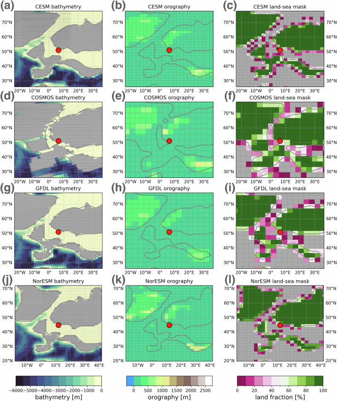
Maps of local boundary condition differences between some of the models around the the Store Bælt (Denmark) site defined in Fig. 4 produced by the web application. Note the different paleogeographic reconstruction used in NorESM (panel j-l).


How to cite the dataset
This Data Descriptor paper should be cited whenever any netCDF files from the dataset or results from the web application are reused in a publication. In addition, the user might want to cite the previously published overview of simulated large-scale climate features13 or the DeepMIP-Eocene experimental design12, as appropriate.
References
Tierney, J. E. et al. Past climates inform our future. Science 370, eaay3701, https://doi.org/10.1126/science.aay3701 (2020).
Hollis, C. J. et al. The DeepMIP contribution to PMIP4: methodologies for selection, compilation and analysis of latest Paleocene and early Eocene climate proxy data, incorporating version 0.1 of the DeepMIP database. Geoscientific Model Development 12, 3149–3206, https://doi.org/10.5194/gmd-12-3149-2019 (2019).
Burke, K. D. et al. Pliocene and Eocene provide best analogs for near-future climates. Proceedings of the National Academy of Sciences 115, 13288–13293, https://doi.org/10.1073/pnas.1809600115 (2018).
Rae, J. W. et al. Atmospheric CO2 over the Past 66 Million Years from Marine Archives. Annual Review of Earth and Planetary Sciences 49, 609–641, https://doi.org/10.1146/annurev-earth-082420-063026 (2021).
Inglis, G. N. et al. Global mean surface temperature and climate sensitivity of the early Eocene Climatic Optimum (EECO), Paleocene-Eocene Thermal Maximum (PETM), and latest Paleocene. Climate of the Past 16, 1953–1968, https://doi.org/10.5194/cp-16-1953-2020 (2020).
Heinemann, M., Jungclaus, J. H. & Marotzke, J. Warm Paleocene/Eocene climate as simulated in ECHAM5/MPI-OM. Climate of the Past 5, 785–802, https://doi.org/10.5194/cp-5-785-2009 (2009).
Roberts, C. D., LeGrande, A. N. & Tripati, A. K. Climate sensitivity to Arctic seaway restriction during the early Paleogene. Earth and Planetary Science Letters 286, 576–585, https://doi.org/10.1016/j.epsl.2009.07.026 (2009).
Winguth, A., Shellito, C., Shields, C. & Winguth, C. Climate Response at the Paleocene-Eocene Thermal Maximum to Greenhouse Gas Forcing-A Model Study with CCSM3. Journal of Climate 23, 2562–2584, https://doi.org/10.1175/2009JCLI3113.1 (2010).
Lunt, D. J. et al. CO2-driven ocean circulation changes as an amplifier of Paleocene-Eocene thermal maximum hydrate destabilization. Geology 38, 875–878, https://doi.org/10.1130/G31184.1 (2010).
Huber, M. & Caballero, R. The early Eocene equable climate problem revisited. Climate of the Past 7, 603–633, https://doi.org/10.5194/cp-7-603-2011 (2011).
Lunt, D. J. et al. A model-data comparison for a multi-model ensemble of early Eocene atmosphere-ocean simulations: EoMIP. Climate of the Past 8, 1717–1736, https://doi.org/10.5194/cp-8-1717-2012 (2012).
Lunt, D. J. et al. The DeepMIP contribution to PMIP4: experimental design for model simulations of the EECO, PETM, and pre-PETM (version 1.0). Geoscientific Model Development 10, 889–901, https://doi.org/10.5194/gmd-10-889-2017 (2017).
Lunt, D. J. et al. DeepMIP: model intercomparison of early Eocene climatic optimum (EECO) large-scale climate features and comparison with proxy data. Climate of the Past 17, 203–227, https://doi.org/10.5194/cp-17-203-2021 (2021).
Anagnostou, E. et al. Proxy evidence for state-dependence of climate sensitivity in the Eocene greenhouse. Nature Communications 11, 4436, https://doi.org/10.1038/s41467-020-17887-x (2020).
Kelemen, F. D. et al. Meridional Heat Transport in the DeepMIP Eocene Ensemble: Non-CO2 and CO2 Effects. Paleoceanography and Paleoclimatology 38, e2022PA004607, https://doi.org/10.1029/2022PA004607 (2023).
Goudsmit-Harzevoort, B. et al. The Relationship Between the Global Mean Deep-Sea and Surface Temperature During the Early Eocene. Paleoceanography and Paleoclimatology 38, e2022PA004532, https://doi.org/10.1029/2022PA004532 (2023).
Zhang, Y. et al. Early Eocene Ocean Meridional Overturning Circulation: The Roles of Atmospheric Forcing and Strait Geometry. Paleoceanography and Paleoclimatology 37, https://doi.org/10.1029/2021PA004329 (2022).
Niezgodzki, I. et al. Simulation of Arctic sea ice within the DeepMIP Eocene ensemble: Thresholds, seasonality and factors controlling sea ice development. Global and Planetary Change 214, 103848, https://doi.org/10.1016/j.gloplacha.2022.103848 (2022).
Williams, C. J. R. et al. African Hydroclimate During the Early Eocene From the DeepMIP Simulations. Paleoceanography and Paleoclimatology 37, https://doi.org/10.1029/2022PA004419 (2022).
Reichgelt, T. et al. Plant Proxy Evidence for High Rainfall and Productivity in the Eocene of Australia. Paleoceanography and Paleoclimatology 37, https://doi.org/10.1029/2022PA004418 (2022).
Cramwinckel, M. J. et al. Global and Zonal-Mean Hydrological Response to Early Eocene Warmth. Paleoceanography and Paleoclimatology 38, e2022PA004542, https://doi.org/10.1029/2022PA004542 (2023).
Abhik, S. et al. Unraveling weak and short South Asian wet season in the Early Eocene warmth. Communications Earth & Environment 5, 133, https://doi.org/10.1038/s43247-024-01289-8 (2024).
Meijer, N. et al. Proto-monsoon rainfall and greening in Central Asia due to extreme early Eocene warmth. Nature Geoscience 17, 158–164, https://doi.org/10.1038/s41561-023-01371-4 (2024).
Kad, P., Blau, M. T., Ha, K.-J. & Zhu, J. Elevation-dependent temperature response in early Eocene using paleoclimate model experiment. Environmental Research Letters 17, 114038, https://doi.org/10.1088/1748-9326/ac9c74 (2022).
Zhang, Z. et al. Impact of Mountains in Southern China on the Eocene Climates of East Asia. Journal of Geophysical Research: Atmospheres 127, https://doi.org/10.1029/2022JD036510 (2022).
Steinig, S. et al. Deep-Time Model Intercomparison Project (DeepMIP) Eocene model data version 1.0, https://doi.org/10.5285/95AA41439D564756950F89921B6EF215 (2024).
Cinquini, L. et al. The Earth System Grid Federation: An open infrastructure for access to distributed geospatial data. Future Generation Computer Systems 36, 400–417, https://doi.org/10.1016/j.future.2013.07.002 (2014).
Iturbide, M. et al. Implementation of FAIR principles in the IPCC: the WGI AR6 Atlas repository. Scientific Data 9, 629, https://doi.org/10.1038/s41597-022-01739-y (2022).
Herold, N. et al. A suite of early Eocene (~55 Ma) climate model boundary conditions. Geoscientific Model Development 7, 2077–2090, https://doi.org/10.5194/gmd-7-2077-2014 (2014).
Baatsen, M. et al. Reconstructing geographical boundary conditions for palaeoclimate modelling during the Cenozoic. Climate of the Past 12, 1635–1644, https://doi.org/10.5194/cp-12-1635-2016 (2016).
Kiehl, J. T. & Shields, C. A. Sensitivity of the Palaeocene-Eocene Thermal Maximum climate to cloud properties. Philosophical Transactions of the Royal Society A: Mathematical, Physical and Engineering Sciences 371, 20130093, https://doi.org/10.1098/rsta.2013.0093 (2013).
Zhu, J., Poulsen, C. J. & Tierney, J. E. Simulation of Eocene extreme warmth and high climate sensitivity through cloud feedbacks. Science Advances 1–11, https://doi.org/10.1126/sciadv.aax1874 (2019).
Hagemann, S. & Dümenil, L. A parametrization of the lateral waterflow for the global scale. Climate Dynamics 14, 17–31, https://doi.org/10.1007/s003820050205 (1998).
Zhang, Z. S. et al. Pre-industrial and mid-Pliocene simulations with NorESM-L. Geoscientific Model Development 5, 523–533, https://doi.org/10.5194/gmd-5-523-2012 (2012).
Schulzweida, U. CDO User Guide. Zenodo https://doi.org/10.5281/zenodo.7112925 (2022).
Hassell, D., Gregory, J., Blower, J., Lawrence, B. N. & Taylor, K. E. A data model of the Climate and Forecast metadata conventions (CF-1.6) with a software implementation (cf-python v2.1). Geoscientific Model Development 10, 4619–4646, https://doi.org/10.5194/gmd-10-4619-2017 (2017).
Rew, R. et al.Unidata NetCDF, https://doi.org/10.5065/D6H70CW6 (1989).
Steinig, S. sebsteinig/deepmip-web-app: as published in DeepMIP data descriptor paper (Scientific Data), https://doi.org/10.5281/ZENODO.12706779 (2024).
Steinig, S. sebsteinig/deepmip-helpers: as published in DeepMIP data descriptor paper (Scientific Data), https://doi.org/10.5281/ZENODO.12706785 (2024).
Zhang, Y. et al. Early Eocene vigorous ocean overturning and its contribution to a warm Southern Ocean. Climate of the Past 16, 1263–1283, https://doi.org/10.5194/cp-16-1263-2020 (2020).
Acknowledgements
Sebastian Steinig and Daniel J. Lunt acknowledge funding from the NERC SWEET grant (grant no. NE/P01903X/1). Daniel J. Lunt also acknowledges funding from NERC DeepMIP grant (grant no. NE/N006828/1) and the ERC (“The greenhouse earth system” grant; T-GRES, project reference no. 340923, awarded to Rich Pancost). The CESM project is primarily supported by the National Science Foundation (NSF). This material is based upon work supported by the National Center for Atmospheric Research, which is a major facility sponsored by the NSF under Cooperative Agreement No. 1852977. Christopher J. Poulsen acknowledges support from the Heising-Simons Foundation (Grant #2016-015) and the National Science Foundation (grant 2309580). MIROC simulations were supported by funding from KAKENHI grant no. 17H06104 and 17H06323. Gordon. N Inglis was supported by a Royal Society Dorothy Hodgkin Fellowship (DHF\R1\191178) and NERC Large Grant (NE/V018388/1). Agatha de Boer and David Hutchinson acknowledge support from Swedish Research Council Grant 2016-03912 and FORMAS grant 2018-0162. The GFDL simulations were performed using resources from the Swedish National Infrastructure for Computing (SNIC) at the National Supercomputer Centre (NSC), partially funded by the Swedish Research Council Grant 2018-05973. Jean-Baptiste Ladant and Yannick Donnadieu acknowledge support form GENCI under allocation A0090102212 to perform the IPSL model simulations with the HPC resources of TGCC.
Author information
Authors and Affiliations
Contributions
The model simulations and individual post-processing were carried out by J.Z. and C.J.P. (CESM), I.N. and G.K. (COSMOS), D.K.H. and A.M.d.B. (GFDL), S.S. and D.J.L. (HadCM3), P.M. and E.M.V. (INMCM), J.B.L. and Y.D. (IPSL), W.L.C. and A.A.O. (MIROC), and Z.Z. (NorESM). D.E., G.N.I. and A.N.M. provided input on the web application and proxy data implementation. S.S. compiled the final dataset and developed the web application. S.S. wrote the manuscript with contributions from all authors.
Corresponding author
Ethics declarations
Competing interests
The authors declare no competing interests.
Additional information
Publisher’s note Springer Nature remains neutral with regard to jurisdictional claims in published maps and institutional affiliations.
Rights and permissions
Open Access This article is licensed under a Creative Commons Attribution 4.0 International License, which permits use, sharing, adaptation, distribution and reproduction in any medium or format, as long as you give appropriate credit to the original author(s) and the source, provide a link to the Creative Commons licence, and indicate if changes were made. The images or other third party material in this article are included in the article’s Creative Commons licence, unless indicated otherwise in a credit line to the material. If material is not included in the article’s Creative Commons licence and your intended use is not permitted by statutory regulation or exceeds the permitted use, you will need to obtain permission directly from the copyright holder. To view a copy of this licence, visit http://creativecommons.org/licenses/by/4.0/.
About this article

Cite this article
Steinig, S., Abe-Ouchi, A., de Boer, A.M. et al. DeepMIP-Eocene-p1: multi-model dataset and interactive web application for Eocene climate research. Sci Data 11, 970 (2024). https://doi.org/10.1038/s41597-024-03773-4
Received:
Accepted:
Published:
DOI: https://doi.org/10.1038/s41597-024-03773-4
This article is cited by
-
Stronger and prolonged El Niño-Southern Oscillation in the Early Eocene warmth
Nature Communications (2025)
