
Abstract
The present study highlights the zeta potential effect of electrokinetic flow in a disk cone system. The study sheds light on the shape of nanoparticles on ternary nanofluid flow with surface catalyzed chemical reaction. The potential implication is optimization of microfluidic appliances and reactors. The pace of reaction on the surface is analyzed by homogeneous and heterogeneous reactions in the presence of surface catalyzed chemical reactions. The designed model is a system of coupled partial differential equations. Utilization of self-similar variables along with normalization converted the system of partial differential equations into ordinary differential equations. Fourth order collocation method by using MATLB helped to analyze the results in graphical form. It has been concluded that electric field parameter, electroosmotic parameter and zeta potential amplifies the radial velocity while disk cone system is rotating in same direction. The lamina shape of the particles is more sensitive to the temperature variation by increasing thermal radiation parameter as compared to spherical shape.
Introduction
In a disk-cone system a unique flow pattern is developed due to counter rotating and co-rotating disk and cone. In the past few years scientists have been scrambling to optimize the microfluidic devices, reactor design, synthesis of chemical and development of pharmaceuticals with disk shaped chamber and cone shape outlet. Gas turbines, which similarly use cone-disk arrangements, use adjustable diffusers to condense air and help cool the system1. Fewell and Hellums2 investigated flow fields, gap angle, and Reynolds number affected disk-cone systems. It has been found that for constant angular velocity the shear force is reduce, and secondary flow is negligible. Sdougos et al.3 used visualization tools and heat transfer probes to test experimentally this result. Shevchuk4 created self-similar solutions, which aided in the study of fluid dynamics and heat transfer in disk-cone systems. With a constant temperature at the cone and fluctuating temperatures throughout the disk, rotationally symmetric and time-independent airflows have been assessed. Velocity and temperature profiles are examined by either component rotated independently, as well as cases in which both rotated in the same or opposing directions.
Notably, all of the research mentioned have looked at circumstances in which either the cone or the disk rotates, or when both components rotate in the same or opposing directions. However, less attention has been paid to the case in which the entire structure remains constant while the fluid is formed to twirl applying an additional twirling mechanism. The scientific community claims that Shevchuk5 was the first to modify the formulas that govern and extract self-similar parameters to replicate fluid movement in a static cone-disk structure. With increased global energy rivalry, improving heat transmission has become a top concern in thermal process areas. Theoretical and experimental research suggests that introducing thermally conductive particles into base fluids improves heat transfer qualities. Maxwell6 first proposed the idea of mixing solids and liquids to improve heat conductivity more over a century ago. Particle sedimentation and agglomeration, caused by increasing particle size and density, are significant problems in many practical cooling applications. Choi7 developed an unusual kind of binary liquids called nanofluids, which were design possible by nanotechnology, in order to address these issues. Nanofluids are created by colloidally floating minuscule elements, for example metallic and oxides, which have a volume percentage of less than 5% and are usually 1–100 nm in diameter, in regular base fluids such water, oil, or biological liquids. Even low concentrations of nanoparticles can drastically modify the thermophysical characteristics of base fluids. For example, choice of nano particles of \(A{l_2}{O_3}\)is based on higher thermal conductivity, inexpensive and availability. And particle of \(Zr{O_2}\)having comparatively low thermal conductivity, but these particles are chemically inert and suitable to synthesize ternary nanofluid. \(CNT\) can be chosen due to highest value of thermal conductivity. Nanofluids, with their increased heat transfer efficiency due to larger surface area and applicability to a wide range of applications, hold significant promise in a variety of sectors. Aside from their functions in tribological and medicinal applications, nanofluids are appreciate in industries that require effective heat removal, such as automotive and nuclear energy. Researchers such as Wang and Majumdar8, Wen et al.9, and Yu and Xie10 have examined nanofluid fabrication methods, characteristics, stability, and application.
The dual-phase speculation, which asserts that nanoparticles are present autonomously within a vehicle liquid, was first forth by Buongiorno11 in 2006. In addition to offering justifications for the enhanced heat transfer observed in nanofluids, the present research highlighted the importance of the speed differential between the fluid being analyze and nanoparticles. When seven escape procedures were investigate in non-turbulent environments, it was discover that thermophoresis and Brownian diffusion had a significant impact. As outcome, four transport equations created especially for nanofluids were included in a two-phase inhomogeneous stability system.
When electrified ionic liquids combine with an electric field, electroosmotic flow (EOF) occurs. By resolving equation of momentum and continuity affected by an additional electronic body power, the equation of Poisson-Boltzmann is frequently use to analyze EOF features in smaller channels and on media like disks or plates. The Debye-Hückel (DH) assumption can use to solve these equations numerically for a variety of structures, flow variables and electrolytes. This approach makes it possible to represent the potential profile explicitly mathematically, particularly for wall of zeta potential that are less than 0.025 V. When current electric field directly given to a permeable substance through electrodes, positively charged electrons drawn to the negatively charged electrode (cathode), causing electroosmosis and electrochemical treatment processes12.
The double-layer charge and the related counterion charge in the void fluid provide an explanation for particle fluidity. Electroosmotic flow (EOF) arises between electrodes because of the cations dragging the pore fluid across the porous substrate and the motion of particles relayed to nearby fluid molecules13. The water removal process boosted by a zone of electric effect, which offers a far higher EOF than a hydraulic field. When dealing with impeded flow materials such fine soils, sediments, and mud, electroosmotic dewatering processes works better than conventional dewatering processes techniques. This approach, first innovated by Casagrande, has been successfully employed in a variety of industrial industries, including soil consolidation, sludge dewatering14, soil remediation15,16, food processing17, metallurgical waste management18,19, and even nuclear applications20. Shajar21 Abbas used the constant proportional Caputo (CPC) fractional operator and Laplace method to see the impact of Hall current on the multiphase thermal transfer of an electrically conductive Jeffery fluid. Mudassar Nazar22 use the fractional calculus and Laplace transform method to explore the unsteady MHD Casson fluid flow across the accelerating porous plate. Mushtaq Ahmed23 exploit the Soret effect across the oscillating plate to study the unsteady MHD Casson fluid flow for introduce the constant proportional Caputo operator. To assess the unsteady Casson fluid across the heat radiation and mass diffusion using Caputo-Fabrizio fractional operator24. Poly Karmakar25,26,27,28,29,30,31,32,33 explores bio electromagnetics in blood circulation and analyze the effect of electroosmosis, heat transfer for the innovation of medical devices.
Reactions of chemicals that take place between substances in an identical phase whether they be liquids, gas, or solids and in which the reactants and products stay in the same state are known as homogeneous reactions. While, heterogeneous reactions take place between substances in different state, including solids and gases, liquids and gases, and solids and liquids. A solid catalyst, which offers a surface for contact with reactant molecules, is extensively use in these reactions to speed up the process. Homogeneous reactions, unlike heterogeneous reactions, rarely require a catalyst because reactants are already sufficiently close within the same phase34.
Ternary nanofluid research has become a developing area of fluid dynamics and thermal science with potential uses in both the commercial and technical domains. Compared to conventional fluids, ternary nanofluids have improved stability and thermal properties by combining three different kinds of nanoparticles with a base fluid. The behavior of CY ternary nanofluid thin films on a rotating porous disk has been the subject of recent studies that have investigated changes in thin film thickness under partial slip situations35.
The above literature survey indicates that envisaged mathematical models give several novel contributions in context of surface catalyzed reaction and electrostatics. It couples the shape effect of nanocomposites in the counter rotating and rotating disk cone system. Debye-Hückel (DH) approximation for electroosmotic effects are studied by using Boltzmann distribution, assuming no overlap of the electric double layer (EDL).The zeta potential enhance the radial velocity and surface catalyzed reactions decrease the concentration profile. The present solution is sought by using BVPs built in MATLAB. However, various numerical schemes24,36,37 are available to solve the highly non-linear problem. But BVP4C is an efficient and more accurate methodology to find the solution of above problem. Table 1 gives the comparison of the effects considered in the present study with the existing literature.
Mathematical formulation
The incompressible movement of a ternary nanofluid between a disk and a cone is explore in cylindrical coordinates, with a focus on electroosmosis, radiant heat, and homogeneous-heterogeneous processes.
The study is conduct under the following assumptions:
-
Assumed the flow is steady in disk cone system.
-
The zeta potential induced by Electrical Double Layer (EDL).
-
External effects are negligible.
-
The surface catalyzed reaction.
-
Analyze effect of ternary fluid and shape factors.
-
The disk has a rotational velocity of in the forward direction, whereas the cone circulates at Ω within the rotational plane. This study eliminates the amount of pressure gradient. Figure 1 shows the axisymmetric fluid flow equations, and the interpretation is perform for three different physical ways:
Fig. 1 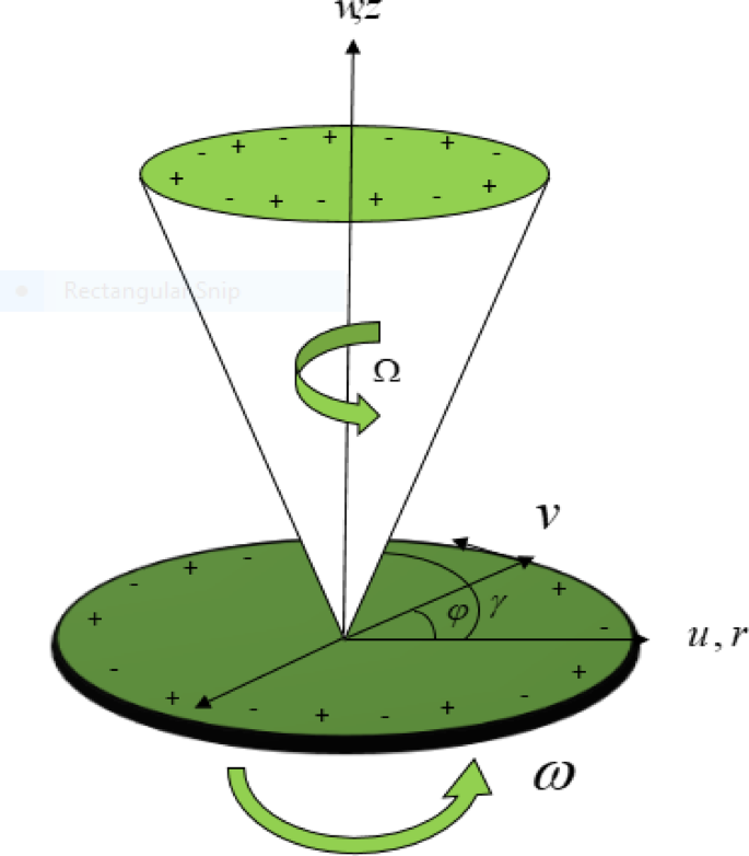
Disk-cone system.

Here are the benchmark cases of the study.
(i) Both the disk and the cone are spinning, i.e. \({\operatorname{Re} _\omega } \ne 0\,\)and \({\operatorname{Re} _\Omega } \ne 0\)(ii) a stationary cone with a revolving disc, i.e. \({\operatorname{Re} _\Omega }=0\)and \({\operatorname{Re} _\omega } \ne 0\)(iii) a rotating cone with a stationary disc, i.e. \({\operatorname{Re} _\Omega } \ne 0\)and\({\operatorname{Re} _\omega }=0\).
Using flow analysis, the homogeneous cubic autocatalytic reaction between species A and B can be examine and is represented below:
A first-order isothermal reaction on a catalyst’s surface is depict in the format below.
The expression uses the rate constants\({k_c}\)and\({k_s}\)with a and b denoting the concentrations of chemical species A and B respectively. Both reaction processes have considered isothermal.
According to the above assumptions the component form of the Eqs34,41,42,43,44,45:
Electrical potential45
Dispersion of electrical potential in the electric double layer (EDL) is explained by the Boltzmann–Poisson Eq.
In this context,\(D(={\varepsilon _{ef}}\overline {\phi } )\), \({\rho _e}\)represents the volume density of change and\({\varepsilon _{ef}}\)is the permittivity of dielectric.
Positioning on the permeable disc’s surface has no effect on the permittivity.
And
In this scenario, \({n^ - }\)and\({n^+}\)signify the densities of anions and cations, both deemed to have a overall concentration of\({n_0}.\)
Thus, the Boltzmann distribution can formulate as follows, considering the electric double layer (EDL) does not coexist.
In this context, \(\overline {e}\)represents the electric charge, \(\overline {{{z_1}}}\)denotes the balance of charge,\({K_B}\)is the Boltzmann constant, and \({K_B}\)corresponds to the usual temperature of the electrolyte solution.
The charge density second order differential equation, for the electric potential distribution is putting into Boltzmann-Poisson Eq.
Boundary conditions34,45,39
Self-similar transformations34,45,39
Self-similar model
The above Eqs. (3)–(9) are change into the following form
After solving Eq. (20) and Eq. (22), we get the following results
The relevant boundary conditions in dimensionless form are:
The diffusion coefficients of species A and B are nearly same, implying that\({D_B}\)and\({D_A}\)are equivalent (represented by\(\delta =1\)). Thus, in accordance with references34,35, we get:
According to this assumption Eq. (24) and Eq. (25) to
With boundary conditions as
The choice of nano particles of \(A{l_2}{O_3}\)is due to the reason that these particles have high thermal conductivity as shown in Table 2, inexpensive and availability. Table 2 indicates that particle of \(Zr{O_2}\)have comparatively low thermal conductivity, but these particles are chemically inert and suitable to synthesize ternary nanofluid. Additionally, these particles are highly stable at extreme temperatures. \(CNT\) are used as nanoparticles having highest value of thermal conductivity as shown in Table 2. These particles have exceptional mechanical strength which make them suitable in extreme temperature environment. The following are the pro and cons of these particles used in Table 2.
Table 3 gives the mathematical expression for thermophysical properties, Table 4 gives the numerical values thermophysical properties. Table 5 gives the values of sphericity values for various shapes of particles.
The dimensionless parameters are used.
In this context \({m^2}\)demonstrate as electroosmosis parameter, \(\Pr\)depict the Prandtl number, parameter of electric field is \({U_e}\), \({U_{HS}}\)indicate the Helmholtz-Smoluchowski velocity, \(Rd\)is the radiation parameter, \({K_{vs}}\)exhibit the surface catalyst, \(Sc\)is the Schmidt number, Q indicate the heat generation parameter, \(\tau\)is the zeta potential.
Nusstle number and skin friction is define as:
Table 6 gives the heat transfer rate in both cases RTC and stationary disk, RTD and stationary cone when Prandtl number vary from 0.1 to1 and \(n=0\) then our results match with the previous studies Shevchuk41 and Wang et al.38.
Solution methodology
The MATLAB Bvp4c method, designed for solving nonlinear equations with boundary conditions, first requires the governing ODEs to be reformulated into a system of first-order ODEs before proceeding with the numerical solution
So the transformed first order equations are
And the transformed boundary conditions are
There are some advantages of BVP4C.
-
BVP4C provides high accuracy and reliable results.
-
It is robust scheme and can handle a wide range of BVPs.
-
It is computationally efficient and can solve BVPs quickly.
-
It is flexible for boundary conditions.
-
It can handle singularities and discontinuities in the solution.
-
It is use in various fields like engineering, physics and biology.
Results and discussion
The influence of key parameters on velocity, temperature and concentration profile is depicted in Figs. 2, 3, 4, 5, 6, 7, 8, 9, 10, 11, 12 and 13. Figure 2 represent the effect of electric field parameter on radial velocity profile. Near the disk, the radial velocity profile is increasing. Moving away from the boundary, the deceleration in radial velocity occurs. Physically, in cone-disk systems, raising the electric field parameter increases Coulomb forces, which directly accelerate charged particles. This increased acceleration mitigates the effects of centrifugal forces and viscous drag, allowing particles to travel radially inward more efficiently. Furthermore, the electric field modifies plasma behavior by reducing resistive forces and increasing radial velocity. As the field strength increases, the inward particle movement becomes more dynamic and fast. Radial inflow is compensated for by the axial outflow.

The fluctuation in radial velocity by\({U_e}\)

The fluctuation in radial velocity by m.

The fluctuation in tangential velocity by\({\operatorname{Re} _\omega }\)and \({\operatorname{Re} _\Omega }\)

The fluctuation in tangential velocity by \({\operatorname{Re} _\Omega }\)and \({\operatorname{Re} _\omega }\)

The fluctuation in radial velocity\(F\left( \eta \right)\) by zeta potential τ

The fluctuation in concentration profile\({\phi _A}\left( \eta \right)\) by\({K_{vs}}\)

The fluctuation in concentration profile\({\phi _A}\left( \eta \right)\) by \({K_2}\)

The fluctuation in concentration profile\({\phi _A}\left( \eta \right)\) by \({K_1}\)

The fluctuation in temperature profile by\(Rd\)

Heat transfer rate for the enhancement of radiation parameter for lamina and spherical shape of particle.

The impact of\({\operatorname{Re} _\omega }\)on heat transfer rate

The impact of\({\operatorname{Re} _\Omega }\)on heat transfer rate
The impact of electroosmosis parameter m on the radial velocity is shown in Fig. 3. The enhancement in radial velocity near the disk and deceleration in fluid motion is witnessed. Physical significance is by increasing the electroosmosis parameter m reduces the Debye length, affecting the distribution of electrical potential, which maintains the flow and alters the force balance. Figure 4 draws the tangential velocity profile, when the cone’s velocity increases while the disk rotates at a constant speed. The enhancement in fluid’s tangential velocity is due to increased shear stresses at the fluid-cone contact. The increased cone velocity imparts additional angular momentum to the fluid, leading to amplifying the rotational motion. Additionally the interaction between the cone’s motion and the fluid layers increases the tangential velocity, resulting in a greater rotating flow field across the system. Figure 5 describes the tangential velocity when the cone moves at a constant speed while the disk accelerates. Similar behavior is observed as shown in Fig. 4. The tangential velocity increases due to improved momentum transfer from the faster-moving disk to the fluid. The increasing speed of disk causes larger shear pressures at the disk-fluid interface, which accelerates the neighboring fluid layers tangentially. This momentum spreads across the flow, resulting in a greater tangential velocity across the system. Figure 6 draws the zeta potential on radial velocity profile. Physically, increase in zeta potential boosts the electric double layer (EDL) effects, leading to more electroosmotic flow. This increases the body force in the radial momentum equation and therefore accelerates the radial velocity. The higher the zeta potential, the greater the driving force for fluid motion due to the increased coupling between the electric field and the fluid. This causes a more prominent radial flow in the system. Figure 7 shows the surface-catalyzed parameter\({K_{vs}}\)on the dimensionless concentration\(\phi \left( \eta \right)\). The results reveal that increasing the surface-catalyzed parameter reduces concentration. The escalating values of surface catalyzed parameter boosts the rate of reaction and therefore the concentration profile declined rapidly. Figures 8 and 9 show the effect of homogeneous and heterogeneous reaction parameters on the concentration profile. Increasing\({K_1}\)and\({K_2}\)decreases mass transfer. As the chemical reaction, parameters increase the rate of reaction increases. Therefore, reactants are transform into the products. Figure 10 manifests the shape factor of nanoparticle for spherical and lamina shape by increasing radiation parameter. It is observed that lamina shape (\(sf=3\)) of particle is more sensitive to the enhancement in radiation parameter as compared to the spherical shape\(sf=16.1576\). The enhancement in radiation parameter will results in the heating of disk cone system. A greater \(Rd\)improves the fluid’s diffusion coefficient, which accelerates heat transfer inside the layer. This leads to increased thermal radiation emission.
Figure 11 depicts a bar chart of heat transfer rates for various radiation parameter values. At the disk, the heat transfer rate increases as the radiation parameter increases, with lamina shapes having a bigger increase than spherical shapes. At the cone, however, the heat transfer rate drops as radiation parameters increase, with spherical shapes showing a larger reduction than lamina shapes.
Figure 12 depicts a bar chart of the heat transfer rate at various local Reynolds number \({\operatorname{Re} _\omega }\) values. At the disk, the heat transfer rate increases as the local Reynolds number \({\operatorname{Re} _\omega }\) grows, with lamina shapes showing a greater increase than spherical shapes. At the cone, the heat transfer rate reduces as the local Reynolds number \({\operatorname{Re} _\omega }\) increases, with spherical geometries seeing a greater decline than lamina shapes.
Figure 13 depicts a bar chart of the heat transfer rate at various local Reynolds number values. At the disk, the heat transfer rate reduces as the local Reynolds number rises, with spherical geometries showing a greater reduction than lamina shapes. In contrast, at the cone, the heat transfer rate increases with greater local Reynolds numbers, with lamina shapes showing a steeper increase than spherical shapes.
Conclusion
To address the challenges in microfluidic devices and various reactors the present mathematical model provides the complex interaction between nanoparticles of \(A{l_2}{O_3}\),\(Zr{O_2}\),\(CNT\) of Lamina and spherical shape in the presence of electroosmotic forces. The key findings are as follows:
-
1.
The radial velocity profile is dependent on electric field parameter. Which clarifies newly developed theoretical frameworks. For example, in Electrostatic flow control in heat exchangers, electrostatic filters and various thermal management devices.
-
2.
Momentum of the flowing fluid is escalating for the rotating disk-cone system which is helpful in the design of rotatory machinery system, turbines and pumps by considering non-Newtonian fluids.
-
3.
The presence of surface catalyzed reaction enhances the rate of reaction. Understanding the reaction kinetics is helpful in electrochemical reactors. It can be further extended to developed newly catalyst materials to obtain maximum reaction rates in various techniques photoelectron spectroscopy and atomic force microscopy.
-
4.
Increase in zeta potential boosts the electric double layer (EDL) effects, leading to more electroosmotic flow. It highlights the importance of zeta potential in electroosmotic flow in electrochemical systems. The study can be further enhanced to simulate EDL dynamics in various electrochemical reactors.
-
5.
The lamina shape of particle is more sensitive to the enhancement in radiation parameter as compared to the spherical shape. This can inform the specific particle shape in chemical processing, radiation therapy and energy production. More non spherical shapes can also be studied\.
Limitations
The some limitations of the study are.
-
Thermophysical properties are consider to be the constant in present study. However, due to temperature variations these properties may varies.
-
It is a theoretical base not an experimental study.
-
This study specific design and shape of disk cone system.
-
The flow behavior is considered to be steady.
Future research directions
There is some future directions are.
-
Thermophysical properties can be considered as a function of temperature. .
-
Unsteady flow behavior can be considered to make problem more innovative.
-
Various more shapes of particles can be studied.
Data availability
The datasets used and/or analysed during the current study available from the corresponding author on reasonable request.
Abbreviations
- \(D_A\) and \(D_B\) :
-
Diffusion coefficient \(\left( {m^2 s^{ - 1} } \right)\)
- \(F\left( \eta \right),G\left( \eta \right),H\left( \eta \right)\) :
-
Velocity profiles
- \(K_1\) :
-
Parameter of homogeneous reaction
- \(K_2\) :
-
Heterogeneous parameter
- \(k_c ,k_s\) :
-
Rate constant
- \(k_f\) :
-
Thermal conductivity \(\left( {Wm^{ - 1} K^{ - 1} } \right)\)
- \(Nu_c\) :
-
Nusselt number at cone surface
- \(Nu_d\) :
-
Nusselt number at disk surface
- \(\Pr\) :
-
Prandtl number
- \(p\) :
-
Pressure \(\left( {N/m^2 } \right)\)
- \(Q_o\) :
-
Heat source \(\left( J \right)\)
- \(Sc\) :
-
Schmidt number
- \(T_b\) :
-
Ambient temperature \(\left( K \right)\)
- \(T_d\) :
-
Surface temperature \(\left( K \right)\)
- \(T\) :
-
Temperature \(\left( K \right)\)
- \(\left( {u,v,w} \right)\) :
-
Velocity components \(\left( {ms^{ - 1} } \right)\)
- \(\left( {r,\phi ,z} \right)\) :
-
Cylindrical coordinates \(\left( m \right)\)
- \(\rho_f\) :
-
Density \(\left( {kgm^{ - 3} } \right)\)
- \(\mu_f\) :
-
Dynamic viscosity \(\left( {kgs^{ - 1} m^{ - 1} } \right)\)
- \(\rho C_p\) :
-
Heat capacitance \(\left( {kgm^{ - 1} s^{ - 2} K^{ - 1} } \right)\)
- \(\phi \left( \eta \right)\) :
-
Profile of dimensionless concentration
- \(\theta \left( \eta \right)\) :
-
Profile of dimensionless temperature
- \(\delta\) :
-
Parameter of rate of mass diffusion
- \(\nu_f\) :
-
Viscosity of kinematics \(\left( {m^2 s^{ - 1} } \right)\)
- \(\operatorname{Re}_\Omega\) and \(\operatorname{Re}_\omega\) :
-
Local Reynolds numbers
- \(\omega ,\Omega\) :
-
Angular velocities of disk and cone \(\left( {s^{ - 1} } \right)\)
- \(f\) \(tnf\) :
-
Fluid Ternary nanofluid
- \(nf\) :
-
Nanofluid
- \(tnf\) :
-
Ternary nanofluid
- \(T_b\) :
-
Ambient temperature \(\left( K \right)\)
- \(D_A\) and \(D_B\) :
-
Diffusion coefficient \(\left( {m^2 s^{ - 1} } \right)\)
- \(Q_o\) :
-
Heat source \(\left( J \right)\)
- \(K_2\) :
-
Heterogeneous parameter
- \(Nu_c\) :
-
Nusselt number at cone surface
- \(Nu_d\) :
-
Nusselt number at disk surface
- \(K_1\) :
-
Parameter of homogeneous reaction
- \(\Pr\) :
-
Prandtl number
- \(\phi \left( \eta \right)\) :
-
Profile of dimensionless concentration
- \(\theta \left( \eta \right)\) :
-
Profile of dimensionless temperature
- \(p\) :
-
Pressure \(\left( {N/m^2 } \right)\)
- \(k_c ,k_s\) :
-
Rate constant
- \(Sc\) :
-
Schmidt number
- \(T_d\) :
-
Surface temperature \(\left( K \right)\)
- \(T\) :
-
Temperature \(\left( K \right)\)
- \(k_f\) :
-
Thermal conductivity \(\left( {Wm^{ - 1} K^{ - 1} } \right)\)
- \(\left( {u,v,w} \right)\) :
-
Velocity components \(\left( {ms^{ - 1} } \right)\)
- \(F\left( \eta \right),G\left( \eta \right),H\left( \eta \right)\) :
-
Velocity profiles
References
Owen, J. M. & Rogers, R. H. Flow and Heat Transfer in Rotating Disc Systems, Vol. 1 (Rotor-Stator systems, 1989).
Fewell, M. E. & Hellums, J. D. The secondary flow of newtonian fluids in cone-and‐plate viscometers. Trans. Soc. Rheology. 21 (4), 535–565 (1977).
Sdougos, H. P., Bussolari, S. R. & Dewey, C. F. Secondary flow and turbulence in a cone-and-plate device. J. Fluid Mech. 138, 379–404 (1984).
Shevchuk, I. V. A self-similar solution of Navier–Stokes and energy equations for rotating flows between a cone and a disk. High Temp. 42 (1), 104–110 (2004).
Shevchuk, I. V. Laminar heat transfer of a swirled flow in a conical diffuser. Self-similar solution. Fluid Dyn. 39 (1), 42–46 (2004).
Maxwell, J. C. A treatise on electricity and magnetism. Clarendon Press. Google Schola. 2, 3408–3425 (1873).
Choi, S. U. & Eastman, J. A. Enhancing thermal conductivity of fluids with nanoparticles (No. ANL/MSD/CP-84938; CONF-951135-29). (Argonne National Lab. (ANL), 1995).
Wang, X. Q. & Mujumdar, A. S. A review on nanofluids-part I: theoretical and numerical investigations. Braz. J. Chem. Eng. 25, 613–630 (2008).
Wen, D., Lin, G., Vafaei, S. & Zhang, K. Review of nanofluids for heat transfer applications. Particuology 7 (2), 141–150 (2009).
Yu, W. & Xie, H. A review on nanofluids: preparation, stability mechanisms, and applications. J. Nanomaterials. 2012 (1), 435873 (2012).
Buongiorno, J. Convective transport in nanofluids. (2006).
Martin, L., Alizadeh, V. & Meegoda, J. Electro-osmosis treatment techniques and their effect on dewatering of soils, sediments, and sludge: A review. Soils Found. 59 (2), 407–418 (2019).
Alshawabkeh, A. N. & Acar, Y. B. Electrokinetic remediation. II: theoretical model. J. Geotech. Eng. 122 (3), 186–196 (1996).
Iwata, M., Tanaka, T. & Jami, M. S. Application of electroosmosis for sludge dewatering—a review. Drying Technol. 31 (2), 170–184 (2013).
Cameselle, C. & Gouveia, S. Electrokinetic remediation for the removal of organic contaminants in soils. Curr. Opin. Electrochem. 11, 41–47 (2018).
Liu, L., Li, W., Song, W. & Guo, M. Remediation techniques for heavy metal-contaminated soils: principles and applicability. Sci. Total Environ. 633, 206–219 (2018).
Menon, A., Mashyamombe, T. R., Kaygen, E., Nasiri, M. S. M. & Stojceska, V. Electro-osmosis dewatering as an energy efficient technique for drying food materials. Energy Procedia. 161, 123–132 (2019).
Lee, J. K., Shang, J. Q. & Xu, Y. Electrokinetic dewatering of mine tailings using DSA electrodes. Int. J. Electrochem. Sci. 11 (5), 4149–4160 (2016).
Cánovas, M., Valenzuela, J., Romero, L. & González, P. Characterization of electroosmotic drainage: application to mine tailings and solid residues from leaching. J. Mater. Res. Technol. 9 (3), 2960–2968 (2020).
Lamont-Black, J., Jones, C. J. & White, C. Electrokinetic geosynthetic dewatering of nuclear contaminated waste. Geotext. Geomembr. 43 (4), 359–362 (2015).
Abbas, S. & Nazar, M. Fractional analysis of unsteady magnetohydrodynamics Jeffrey flow over an infinite vertical plate in the presence of hall current. Math. Methods Appl. Sci. 48 (1), 253–272 (2025).
Abbas, S. et al. Effect of chemical reaction on MHD Casson natural convection flow over an oscillating plate in porous media using Caputo fractional derivative. Int. J. Therm. Sci. 207, 109355 (2025).
Abbas, S. et al. Soret effect on MHD Casson fluid over an accelerated plate with the help of constant proportional Caputo fractional derivative. ACS Omega. 9 (9), 10220–10232 (2024).
Abbas, S. et al. Application of heat and mass transfer to convective flow of Casson fluids in a microchannel with Caputo–Fabrizio derivative approach. Arab. J. Sci. Eng. 49 (1), 1275–1286 (2024).
Karmakar, P. & Das, S. A neural network approach to explore bioelectromagnetics aspects of blood circulation conveying tetra-hybrid nanoparticles and microbes in a ciliary artery with an endoscopy span. Eng. Appl. Artif. Intell. 133, 108298 (2024).
Das, S., Karmakar, P. & Ali, A. Electrothermal blood streaming conveying hybridized nanoparticles in a non-uniform endoscopic conduit. Med. Biol. Eng. Comput. 60 (11), 3125–3151 (2022).
Karmakar, P., Ali, A. & Das, S. Circulation of blood loaded with trihybrid nanoparticles via electro-osmotic pumping in an eccentric endoscopic arterial Canal. Int. Commun. Heat Mass Transfer. 141, 106593 (2023).
Das, S., Karmakar, P. & Ali, A. Simulation for bloodstream conveying bi-nanoparticles in an endoscopic Canal with blood clot under intense electromagnetic force. Waves Random Complex. Media, 1–38. (2023).
Karmakar, P. & Das, S. Electro-blood circulation fusing gold and alumina nanoparticles in a diverging fatty artery. BioNanoScience 13 (2), 541–563 (2023).
Karmakar, P. & Das, S. Modeling non-Newtonian magnetized blood circulation with tri-nanoadditives in a charged artery. J. Comput. Sci. 70, 102031 (2023).
Karmakar, P., Barman, A. & Das, S. EDL transport of blood-infusing tetra-hybrid nano-additives through a cilia-layered endoscopic arterial path. Mater. Today Commun. 36, 106772 (2023).
Karmakar, P. & Das, S. EDL induced electro-magnetized modified hybrid nano-blood circulation in an endoscopic fatty charged arterial indented tract. Cardiovasc. Eng. Technol. 15 (2), 171–198 (2024).
Karmakar, P., Das, S., Mahato, N., Ali, A. & Jana, R. N. Dynamics prediction using an artificial neural network for a weakly conductive ionized fluid streamed over a vibrating electromagnetic plate. Eur. Phys. J. Plus. 139 (5), 407 (2024).
He, Z. et al. Theoretical exploration of heat transport in a stagnant power-law fluid flow over a stretching spinning porous disk filled with homogeneous-heterogeneous chemical reactions. Case Stud. Therm. Eng. 50, 103406 (2023).
Alipour, N., Jafari, B. & Hosseinzadeh, K. Thermal analysis and optimization approach for ternary nanofluid flow in a novel porous cavity by considering nanoparticle shape factor. Heliyon 9 (12). (2023).
Abbas, S. et al. Heat and mass transfer through a vertical channel for the Brinkman fluid using prabhakar fractional derivative. Appl. Therm. Eng. 232, 121065 (2023).
Abbas, S. et al. Analysis of fractionalized Brinkman flow in the presence of diffusion effect. Sci. Rep. 14 (1), 22507 (2024).
Wang, F. et al. The effects of nanoparticle aggregation and radiation on the flow of nanofluid between the gap of a disk and cone. Case Stud. Therm. Eng. 33, 101930 (2022).
John, A. S., Mahanthesh, B. & Shevchuk, I. V. Study of nanofluid flow and heat transfer in a stationary cone-disk system. Therm. Sci. Eng. Progress. 46, 102173 (2023).
Manjunatha, S. et al. Influence of non-linear thermal radiation on the dynamics of homogeneous and heterogeneous chemical reactions between the cone and the disk. High Temp. Mater. Processes (London). 43 (1), 20240052 (2024).
Shevchuk, I. V. Laminar heat and mass transfer in rotating cone-and-plate devices. (2011).
Shevchuk, I. V. An asymptotic expansion method vs a self-similar solution for convective heat transfer in rotating cone-disk systems. Phys. Fluids, 34 (10). (2022).
Shevchuk, I. V. Convective Heat and Mass Transfer in Rotating Disk Systems, Vol. 45, 1–239 (Springer, 2009).
Basavarajappa, M. & Bhatta, D. Study of flow of Buongiorno nanofluid in a conical gap between a cone and a disk. Phys. Fluids, 34 (11). (2022).
Balaji, R., Prakash, J., Tripathi, D. & Anwar Bég, O. Heat transfer and hydromagnetic electroosmotic von Kármán swirling flow from a rotating porous disc to a permeable medium with viscous heating and joule dissipation. Heat. Transf. 52 (5), 3489–3515 (2023).
Khan, W. A. & Pop, I. M. Effects of homogeneous–heterogeneous reactions on the viscoelastic fluid toward a stretching sheet. (2012).
Bachok, N., Ishak, A. & Pop, I. On the stagnation-point flow towards a stretching sheet with homogeneous–heterogeneous reactions effects. Commun. Nonlinear Sci. Numer. Simul. 16 (11), 4296–4302 (2011).
Alharbi, K. A. M. et al. Computational valuation of Darcy ternary-hybrid nanofluid flow across an extending cylinder with induction effects. Micromachines 13 (4), 588 (2022).
Alshahrani, S. et al. Numerical simulation of ternary nanofluid flow with multiple slip and thermal jump conditions. Front. Energy Res. 10, 967307 (2022).
Arif, M., Kumam, P., Kumam, W. & Mostafa, Z. Heat transfer analysis of radiator using different shaped nanoparticles water-based ternary hybrid nanofluid with applications: A fractional model. Case Stud. Therm. Eng. 31, 101837 (2022).
Chatterjee, D., Biswas, N., Manna, N. K. & Sarkar, S. Effect of discrete heating-cooling on magneto-thermal-hybrid nanofluidic convection in cylindrical system. Int. J. Mech. Sci. 238, 107852 (2023).
Funding
This work was supported and funded by the Deanship of Scientific Research at Imam Mohammad Ibn Saud Islamic University (IMSIU) (grant number IMSIU-DDRSP2503).
Author information
Authors and Affiliations
Contributions
S. R, gave the conceptualization, C. M interpreted the results , A.K simulated the results, S. B investigated the results , N. H. A reviewed the results, B. M. A wrote the introduction, L. K obtain the numerical results.
Corresponding author
Ethics declarations
Competing interests
The authors declare no competing interests.
Additional information
Publisher’s note
Springer Nature remains neutral with regard to jurisdictional claims in published maps and institutional affiliations.
Electronic supplementary material
Below is the link to the electronic supplementary material.
Rights and permissions
Open Access This article is licensed under a Creative Commons Attribution-NonCommercial-NoDerivatives 4.0 International License, which permits any non-commercial use, sharing, distribution and reproduction in any medium or format, as long as you give appropriate credit to the original author(s) and the source, provide a link to the Creative Commons licence, and indicate if you modified the licensed material. You do not have permission under this licence to share adapted material derived from this article or parts of it. The images or other third party material in this article are included in the article’s Creative Commons licence, unless indicated otherwise in a credit line to the material. If material is not included in the article’s Creative Commons licence and your intended use is not permitted by statutory regulation or exceeds the permitted use, you will need to obtain permission directly from the copyright holder. To view a copy of this licence, visit http://creativecommons.org/licenses/by-nc-nd/4.0/.
About this article

Cite this article
Riasat, S., Maatki, C., Kousar, A. et al. Electrical double layer induced zeta potential effect in a disk cone system with surface catalyzed reaction. Sci Rep 15, 16464 (2025). https://doi.org/10.1038/s41598-025-00637-8
Received:
Accepted:
Published:
DOI: https://doi.org/10.1038/s41598-025-00637-8
