
Abstract
Slope instability is a prevalent dynamic disaster encountered in the construction of geotechnical engineering projects. Intelligent detection and early warning systems serve as crucial measures for preventing and controlling slope instability. To accurately and efficiently predict the stability state of slopes, we propose a combined model that integrates the Newton–Raphson optimization algorithm (NRBO) with an optimized extreme gradient boosting tree (XGBoost). Firstly, the primary factors influencing slope instability are thoroughly analyzed. The sample outline is standardized utilizing polar deviation, and the distribution of sample classes is balanced through the application of the Synthetic Minority Over-sampling Technique (SMOTE). Secondly, the XGBoost model is optimized by fine-tuning parameters such as maximum depth (max_depth), learning rate (learning_rate), subsample rate, column sampling rate (colsample-bytree), and minimum loss (gamma) through NRBO. The stability of the model was assessed using a ten fold cross validation method, while the prediction results were comprehensively evaluated utilizing metrics including accuracy (Acc), precision (Pre), recall (Rec), F1 score (Fs), and Cohen’s Kappa coefficient (Ka). Finally, the SHAP additive interpretation method is employed to elucidate the significance and contributions of features influencing the XGBoost model. This model is subsequently applied to ten specific engineering case studies. The results show that after NRBO optimization, the optimal values for the maximum depth, learning rate, subsample proportion, column sample proportion, and minimum loss of the XGBoost model are 7, 0.8247, 0.6326, 0.6263, and 0.0758, respectively. Based on the SHAP model analysis, the main factors influencing the stability of the slopes are g, c, φ, H, and j.
Introduction
As large-scale geotechnical construction grows rapidly, the construction of complex geologic environments inevitably involves mixed slopes, leading to a high trend of landslide geohazards1. Slope instability refers to the sliding or collapse of rock and soil masses triggered by excavation, rainfall, or seismic activity. Its progression involves the coupling of nonlinear geological failure mechanisms, dynamic stress redistribution, and external disturbances2,3. According to statistical data on major non-coal mine accidents in China in 20174, the number of accidents and fatalities caused by slope landslides in mining safety incidents has been steadily decreasing from 2013 to 2017. These incidents ranked third among all mining safety accidents, accounting for approximately 13.5% of total accidents and 9.3% of fatalities. However, with the continuous expansion of large-scale infrastructure projects in China’s geotechnical engineering sector, the frequency of slope instability disasters has significantly increased due to the combined effects of complex geological conditions and intensive engineering activities. This has become a major challenge to engineering safety. Therefore, finding accurate and efficient methods for predicting slope stability is crucial for preventing slope instability and implementing targeted preventive and control measures in advance.
Slope stability prediction is one of the most effective measures to prevent and control the early occurrence of slope instability disasters. Many scholars classify slope stability prediction methods into qualitative and quantitative approaches5,6. The qualitative analysis method involves a comprehensive evaluation of the geometric characteristics, geological structure, hydrological conditions, and regional geological history of the slope to assess its stability and future trends. Examples of such methods include the engineering geological analogy, structural analysis, geological analysis, and graphical methods7,8,9. In contrast, quantitative analysis methods assess the factor of safety and probability of instability of slopes through mathematical models and computational techniques, which include limit equilibrium methods10 and numerical analysis methods11. For example, Deressa et al.12 explored the step geometry and blasting design parameters of open pit limestone mines and proposed a comprehensive optimization framework based on rock properties, equipment constraints and economic objectives. Bezie et al.13 studied high and steep slopes in limestone quarries of cement factories, assessing their stability through geological investigations, kinematic analysis, limit equilibrium methods, and numerical analysis. Hussen et al.14 used a finite element numerical method based on finite element numerical simulation to simulate various rainfall patterns by analyzing slope sections at different saturation levels to assess the stability of failure prone slopes. Although the aforementioned methods provide some insight into predicting slope stability, qualitative analysis methods rely heavily on the experience and intuition of engineering geologists, lack quantitative metrics, and require extensive historical data. Traditional quantitative methods, on the other hand, are based on idealized constitutive assumptions and have limited capacity for handling parameter uncertainties. Moreover, the applicability of both qualitative and traditional quantitative analysis methods is restricted by the small engineering scale and the geological complexity of slope environments. As a result, it is challenging to establish a unified analysis approach that delivers optimal prediction results15,16,17.
In recent years, the rise of new fields such as artificial intelligence has introduced intelligent decision-making as a promising approach for solving complex, nonlinear, and multivariate problems. Many scholars have integrated slope stability prediction indicators into artificial intelligence models. For example, Abolfazl et al.18 employed an integrated approach that combines artificial intelligence and statistical modeling to predict the stability of earth and rock dam slopes.and improved the reliability and accuracy of predicting slope stability by enhancing data driven. Zhang et al.19 integrated three heterogeneous types of information microseismicity, stress, and displacement, both inside and on the surface of the slope along with the Gradient Boosting Decision Trees (GBDT) model to fuse multi-source monitoring data for slope stability prediction. This methodology not only enhanced the model’s capacity to capture intricate nonlinear relationships but also facilitated the prediction of safety factors for open pit mine slopes. Fu et al.20 developed an evaluation model for predicting the stability of slopes based on the Chinese slope rock mass classification system and the principles of Convolutional Neural Networks (CNN). This model demonstrated higher accuracy and better generalization compared to traditional semi-quantitative methods for slope stability prediction.Although these prediction methods can be effective for slope stability prediction, they face certain limitations in practical applications due to the complex mechanisms of slope instability and the inherent shortcomings of various intelligent algorithms. For instance, statistical models typically rely on linear or simple nonlinear assumptions, which can struggle to capture the intricate nonlinear relationships among influencing factors, potentially leading to failure when these assumptions do not hold. The GBDT model depends heavily on feature engineering and suffers from limitations in generalization efficiency and scalability. CNN model training requires significant computational resources, increases engineering costs, and is prone to overfitting when dealing with complex data21,22. Meanwhile, the above methods all have high requirements for the quality and quantity of input data, as well as poor model interpretability and difficulty in handling unstructured data.
In view of this, 221 sets of slope engineering case data were selected to establish initial samples for predicting slope stability. The quality and applicability of the data were enhanced through preprocessing techniques. By combining the Newton Raphson Based Optimizer (NRBO), which offers fast convergence and strong scalability, with the efficient parallel computing and low overfitting risk of eXtreme Gradient Boosting (XGBoost), the model was introduced for slope stability state prediction. The internal feature contributions of the model were analyzed using the additive explanations (SHAP) method. Additionally, the prediction results of this model were compared and analyzed against those of three other models to improve the accuracy of slope stability state prediction and enhance safety in production.
Slope stability prediction mechanism
SMOTE algorithm
The main methods for dealing with data imbalance are under sampling and oversampling. Among them, random under sampling is a direct solution that can remove samples from majority class, but may lose relevant information, leading to a decrease in model accuracy. Conversely, random oversampling increases the minority class by replicating samples, which risks overfitting23. In response to the problem of unbalanced data categories, this article uses the Synthetic Minority Class Oversampling Technique (SMTOE) to insert synthetic samples between the minority class samples, thus resolving the unbalanced data category problem24. The synthesis example is shown in Fig. 1.

Example of SMOTE synthesis.
NRBO algorithm
The proposed NRBO algorithm by Sowmya et al.25 in 2024 is a meta-heuristic optimization technique based on the Newton–Raphson Method (NRM). The algorithm mimics human problem-solving reasoning and improves solution optimization by using Newton–Raphson Search Rule (NRSR) and Trap Avoidance Operator (TAO). For the nth individual in iteration t, the individual’s position is determined using the NRSR, with the new position represented as follows.
where r1 is the random number in (0,1). \({\varvec{X}}_{1n}^{t - 1}\),\({\varvec{X}}_{2n}^{t - 1}\) and \({\varvec{X}}_{3n}^{t - 1}\) are the new vector positions obtained by updating \(x_{n}^{t}\), expressed as.
where Ns is the value obtained by the NRSR search rule. ρ is the step factor. xb is optimal position. δ is an adaptive coefficient.
TAO generates a new solution \(x_{TAO}^{t - 1}\) by combining the optimum position xb and the current vector position \(x_{n}^{t}\), as illustrated below.
where θ1 and θ2 are random numbers uniformly between (− 1,1) and (− 0.5,0.5), respectively; ξ1 and ξ2 are generated equation.
where α is a binary number, representing 1 or 0. If ∆ ≥ 0.5, α = 0, otherwise α = 1. rand is a random number in (0,1).
XGBoost model
Traditional GBDT relies only on first order derivatives for optimization and lacks regularization. In contrast, XGBoost incorporates second-order derivative optimization, introduces regularization terms, and employs distributed computing techniques. These enhancements significantly improve both model performance and computational efficiency26,27. During the training process, XGBoost iteratively adds regression trees to capture the residuals from previous predictions through adaptive optimization strategies, ultimately resulting in a robust learner. The training process is shown in Fig. 2.

XGBoost algorithm flow.
The objective function of the XGBoost model consists of a regularization term and an error term. While the regularization term indicates the structural complexity of the model, the error term indicates the difference between the predicted and actual results. The objective function is formulated as follows.
where: N denotes the total number of slope case samples. l represents the loss function. yi indicates the measured value of the ith sample. \(\hat{y}\) signifies the predicted output of the model. Ω refers to the regularization term associated with the tth tree. γ denotes the learning rate. T represents the current total number of leaf nodes in the regression tree. λ is referred to as a hyperparameter, and ωi denotes the weight assigned to each leaf node.
ROC curve
The Receiver Operating Characteristic (ROC) curve serves as visualization tool for assessing model performance, primarily aimed at quantifying a model’s discriminatory capability through the Area Under the Curve (AUC). In the context of slope stability evaluation, the false positive rate is represented on the x-axis, indicating instances of incorrect predictions regarding slope stability states. Conversely, real positivity rates are plotted along the y-axis, reflecting accurate predictions of these conditions28.
SHAP model
The SHAP model, proposed by Lundberg and Lee29, serves as an attribution explanation method grounded in cooperative game theory. Its fundamental concept concerns the calculation of the contribution of the margins of each feature and its interaction in the model by means of the Shapley value. The Shapley value of a particular feature i can be calculated by averaging the marginal contribution of feature i to all feature subsets Z of the feature set N30. The calculation process is as follows.
where: φi is the Shapley value of the ith input value. f is the original prediction model. |Z| represents the cardinality of set Z. p denotes the total number of features. f (Z ∪ {i}) is a prediction that contains all the features in the {i} subset. f(Z) is a prediction that does not contain all features of {i} subset Z.
Sample selection and data analysis
Sample selection
In essence, slope stability constitutes a complex nonlinear problem influenced by a multitude of factors that can generally be categorized into internal and external causes. Internal factors primarily encompass topography and geomorphology, geological structure, and soil properties. Conversely, external factors predominantly include anthropogenic engineering activities, environmental conditions, and groundwater dynamics. Therefore, with the theoretical studies and engineering experiences related to slope instability, this paper identifies six key factors influencing the slope rock mass from the perspectives of slope structural parameters and geotechnical mechanical and physical properties31. These factors include unit weight (γ), cohesion (c), internal friction angle (φ), slope angle (θ), slope height (H), and pore pressure ratio (ru), which are selected as the input parameters for the proposed combined model. Based on the above slope stability prediction indicators, the author collected 221 groups of typical slope case data to establish the original sample32,33,34,35, and took the actual slope instability as the decision attribute set to establish the initial decision sample data, where F represents the slope instability, S represents the slope stability. See Table 1 for detailed data.
Data analysis
Analysis of indicators
The slope case data samples collected in this paper are independent of each other, where g, c, j, φ, H and ru are the independent variables of the model, and MR is the dependent variable of the model. See Table 2 for the basic information of variables.
As can be seen from Table 2, the means of the c, H, and ru predictors are larger than their corresponding medians and multinomials, so they show a right-skewed distribution. However, the means of g, j and φ predictors are larger than their corresponding medians and plurals, so they show left-skewed distributions. The distribution ranges and frequencies of the variables are shown in Fig. 3.

Distribution curve and interval frequency of each prediction index.
Unbalance analysis
Data imbalance may cause a model to exhibit a bias towards the majority class during training, consequently neglecting or misinterpreting the characteristics of the minority class. The sample number of original slope state distribution is shown in Table 3, and the actual slope state distribution is shown in Fig. 4. From Table 3 and Fig. 4, it can be observed that the number of slope instability samples is 97, accounting for 43.9%, and the number of slope stability samples is 124, accounting for 56.1%. There is a certain imbalance in the sample, so it is necessary to expand a few categories of data to improve the balance of the distribution of each category of the data set.

Actual slope state distribution.
Data processing
Standardized treatment
Because the slope stability prediction indexes are all numerical data, and there are obvious differences in the value range and magnitude of each index. In to increase prediction accuracy of the classification model, polar deviation standardization is used before feature extraction to map the original data to the interval [0,1], eliminating the differences between the data of different dimensions. The standardized data is shown in Table 4.
Unbalance treatment
Since the ratio of samples representing different slope stability states is 1:1.278, it is necessary to balance the various sample types. To achieve this balance, we employ the SMOTE algorithm to augment the samples classified as slope instability. This approach aims to enhance the equilibrium of the state distribution among slope stability samples. The results are shown in Fig. 5.

Comparison between the original sample and the balanced sample.
It can be observed from Fig. 7 that following the expansion of the original samples, the quantities for both slope instability and slope stability have reached 124, and the total number of samples has increased from 221 to 248 groups, which solves the imbalance of sample grade distribution and meets the requirements of machine learning algorithm for sample balance. The sample distribution of each indicator after balance is shown in Fig. 6.

Sample distribution after equilibrium.
Model construction
Algorithm verification
For evaluating the optimization performed by the NRBO algorithm, the authors chose four classical complex nonlinear benchmark functions as test cases for the iterative analysis. The results were compared and analyzed alongside two other algorithms: Differentiated Creative Search (DCS) and PID-based Search Optimization Algorithm (PSA). In this study, the population size of the algorithms was established at 20, while the maximum number of iterations was set to 500. For NRBO, the TOA determinant was established at DF = 0.6. In contrast, for PSA, the proportional coefficient was set to 1, while the integral coefficient was assigned a value of 0.5 and the differential coefficient was determined to be 1.2. The results of the function test are shown in Fig. 7.

Function test results.
It can be seen from Fig. 7 that the NRBO algorithm shows good convergence ability and speed in both single peak and multi peak benchmark test functions, and its convergence ability is significantly improved compared with DCS and PSA algorithms. It is evident that the algorithm demonstrates efficient exploratory capability, rapid convergence speed, and robust optimization performance.
NRBO-XGBoost combination model
XGBoost model has efficient training speed, strong extensibility and better prediction effect, but it takes up a large amount of computing resources and is vulnerable to the influence of super parameter selection. Low memory space and different combinations of super parameters may lead to different prediction results. To accurately and efficiently predict the stability of slopes in geotechnical engineering, the author employs the NRBO algorithm to optimize five critical parameters of the XGBoost model: maximum depth (max_depth), learning rate (learning_rate), subsample ratio (subsample), column sample ratio (colsample_bytree), and minimum loss (gamma). The specific implementation steps for the combined prediction model of geotechnical slope stability, optimized by XGBoost based on the NRBO algorithm, are outlined as follows.
-
a)
Data preprocessing. (1) The range of data distribution is reduced by standardizing the dimensions of unified data to eliminate the deviation of model prediction effect caused by data of different dimensions. (2) SMOTE algorithm is used to deal with the number of samples of slope instability, so that the two types of samples can reach a balance.
-
b)
NRBO initialization. Set the determination factor (TAO) to 0.6. The initial population size (pop_size) is 20. Set the maximum iteration threshold (max_iter) to 100. Set five super parameter optimization intervals.
-
c)
Find the best ___location. Optimization-seeking parameters are introduced into the objective function to update the fitness, the locations of the populations are refreshed according to the current state of the populations and the search rules, and the optimal solutions are updated using the root mean square error as a fitness function. After each iteration, the current optimal solution is used as a reference point for generating subsequent populations, and the fitness of each solution in the current population is evaluated until the stopping condition is recognized and the optimal parameter combination is output.
-
d)
Testing and application. The best combination of parameters after NRBO algorithm optimization is input into XGBoost model, and the best prediction model after training is obtained. The overall process of NRBO-XGBoost slope stability prediction model is shown in Fig. 8.
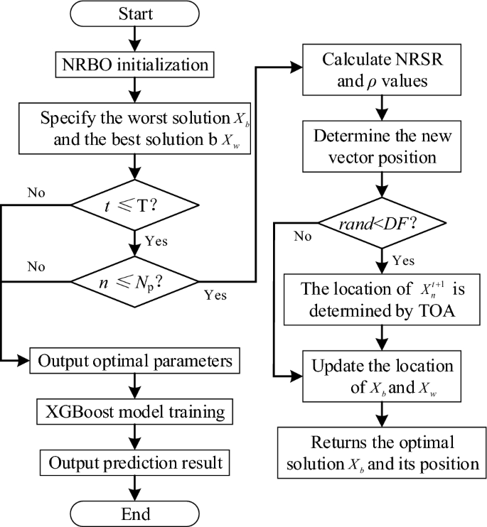
Flow of NRBO-XGBoost prediction model.
Model training and testing
Optimization of model parameters
After establishing the geotechnical engineering slope stability prediction model, 80% of the data from the original samples were randomly selected as the training set to train the model, while the remaining 20% were used as the test set to evaluate the model’s prediction performance. The training set consists of 198 samples, and the test set contains 50 samples, allowing for an assessment of the model’s feasibility, effectiveness, and robustness. Before super parameter optimization, it is necessary to comprehensively analyze the optimized super parameters and value range, as shown in Table 5.
The five hyperparameters of XGBoost model are optimized by NRBO algorithm to find the most suitable combination of hyperparameters with this model, and the dimension of NRBO algorithm is set to 5. Meanwhile, DCS and PSA are introduced to optimize the XGBoost model respectively, and compare the fitness situation of the above three algorithms individually. The results are illustrated in Fig. 9.

Fitness iteration curves for 3 optimization algorithms.
From Fig. 9, it is observed that the NRBO algorithm and DCS algorithm achieve a convergence value of 0.02 after 7 and 20 iterations for optimizing the hyperparameters of the XGBoost model, respectively, while the PSA algorithm requires 28 iterations to achieve a convergence value of 0.05. In contrast, the PSA algorithm requires 28 iterations to reach a higher convergence value of 0.05. This indicates that NRBO not only demonstrates superior optimization performance but also achieves lower convergence values compared to other intelligent algorithms. After optimization, the super parameter combination of the XGBoost model optimized by NRBO is learning_rate = 0.8247, max_depth = 7, sample = 0.6326, colsample_bytree = 0.6263 and gamma = 0.0758.
Model performance evaluation indicators
To validate the performance of the XGBoost slope stability prediction model after optimizing the NRBO algorithm, five metrics, namely Accuracy (Acc), Precision (Pre), Recall (Rec), F1 Score (Fs), and Coenkapa’s Coefficient (Ka), were introduced as a basis for evaluating the model performance35. The calculation process is as follows.
where TP is the true case. TN is the true negative case. FP is the false positive case. FN is the false negative case. N is the total number of samples. n is the total number of sample categories.
Prediction effect analysis
To investigate further the robustness, superiority and robustness of the XGBoost slope stability prediction model optimized by the NRBO algorithm, the accuracy of the constructed model was evaluated in this study using the tenfold cross-validation method. The unoptimized XGBoost model as well as three models using DCS algorithm and PSA algorithm to optimize XGBoost respectively are selected and compared with the model built in the paper to analyze the difference in performance. The prediction performance of each model on the test set is shown in Table 6.
From Table 6, it can be seen that NRBO-XGBoost model predicts the slope stability compared with the actual stability, which is completely consistent with the actual state in the stable state of the slope, while there is a certain deviation in the destabilized state of the slope. It demonstrates that the model built in the paper has strong classification performance for the stable state of the slope and weak classification performance for the unstable state of the slope. Compared with the other 3 models, the NRBO-XGBoost model predicts the most correct slope stability state, which is 46, while DCS-XGBoost and PSA-XGBoost models were followed by 45 and 43 respectively, and the unoptimized XGBoost model predicted the least, 39. In order to intuitively understand the advantages of NRBO-XGBoost model, the comparison thermodynamic diagram of each evaluation index is drawn, as shown in Fig. 10.

Comparison of evaluation indicators of each prediction model.
It can be observed from Fig. 10 that the accuracy of NRBO-XGBoost slope stability accuracy model was increased by 2%, 6% and 14%, the precision was increased by 3.2%, 7.21% and 15.06%, the recall rate was increased by 1.9%, 5.93% and 14%, the F1-score was increased by 1.98%, 6% and 13.96%, and the Cohen’s Kappa coefficient was increased by 4.06%, 12.09% and 19%, respectively, compared with the evaluation indexes of DCS-XGBoost, PSA-XGBoost and XGBoost models. It is evident that the evaluation metrics of the NRBO-XGBoost slope stability prediction model surpass those of alternative models, indicating that this model demonstrates superior accuracy in predicting slope stability. To further verify the performance differences of the prediction models, the ROC curves and AUC values of NRBO-XGBoost, DCS-XGBoost, PSA-XGBoost and XGBoost slope stability prediction models are drawn, as shown in Fig. 11.

ROC curve of each model.
It is evident from Fig. 11 that the ROC curve of the NRBO-XGBoost slope stability prediction model is significantly extended towards the upper left corner, with an AUC value of 0.92 for the area under the curve. The ROC curves for the DCS-XGBoost and PSA-XGBoost prediction models show a secondary level of expansion, with AUC values of 0.90 and 0.85, respectively. In contrast, the non-optimized XGBoost prediction model exhibited the least favorable performance, achieving an AUC value of only 0.78. This analysis indicates that the NRBO-XGBoost model demonstrates superior predictive capability compared to other intelligent algorithm-based prediction models, which exhibit comparatively weaker performance.
Analysis of influencing factors
The causes of slope stability prediction are complex, and it is very important to identify the dominant disaster causing factors for the effective prevention and control strategy of slope instability. For this reason, the author uses the SHAP model to explain the importance of the six impact factors of the XGBoost model. The ranking of feature importance and the summary figure are shown in Fig. 12.

Feature importance ranking and overview.
Figure 12a shows the sequence of characteristic importance of slope stability state prediction, in which g, c, φ, H and j are the main factors affecting slope stability state, while ru has little effect. Each point in Fig. 12b represents a real sample, and the color of the point can reflect the size of the influencing factor value. According to the Shapley value of the given sample and the corresponding eigenvalue, the influence of the feature on the prediction result can be estimated. From a horizontal perspective, taking the influencing factors of g and c as examples, the sample distribution appears relatively scattered. This indicates that the influence of g and c on the model’s prediction results is substantial. In contrast, the influence factors φ, H, j, and ru are more concentrated, suggesting that their impact on the model’s prediction outcomes is comparatively minor. From a vertical standpoint, higher values of φ, h, and ru correspond to greater Shapley values. This implies that these factors have a more significant positive effect on predicting slope stability. Conversely, larger values of g, c, and j are associated with lower Shapley values; this indicates that these factors exert a stronger negative influence on predictions regarding slope stability. To sum up, the selected prediction indicators in this paper have an impact on slope instability, focusing on the influencing factors of g, c, φ, H and j, which can effectively prevent slope instability disasters to a large extent.
Engineering application
In regard to validating the universality and stability of the NRBO-XGBoost slope stability state prediction model, Zhongyancun landslide, sujiaping landslide, Daxi landslide, Zihong reservoir right bank landslide, Xunyang hydropower station yangdagou landslide, Jiangxi Qiyi reservoir landslide, Tianshengqiao cascade II Hydropower Station No. 7 slope, Sichuan kuaoliangzi slope, Yunnan Touzhaigou slope, and the Huanglashi landslide in the Three Gorges of the Yangtze River are taken as specific project case data for verification as external test sets. See Table 7 for specific data. The prediction results and confusion matrix of each model are shown in Figs. 13 and 14.

Prediction results of each model.

Results of rock burst confusion matrix for each model.
From Fig. 13, it can be observed that the NRBO-XGBoost slope stability prediction model has the best fit for each assessment index compared to other intelligent algorithm models, with an accuracy of 90%, the DCS-XGBoost and PSA-XGBoost prediction models have the second highest accuracy of 80%, and the XGBoost model has the worst prediction effect, with an accuracy of 70%. According to the analysis in Fig. 14, the NRBO-XGBoost model mispredicted one sample in predicting the slope stability state, overestimating the slope instability state. However, the prediction effect of DCS-XGBoost and PSA-XGBoost models is slightly poor, and both of them mispredicted two samples. XGBoost model has the highest error rate and mispredicted three samples. In summary, the NRBO-XGBoost model predicts the slope stability state can deeply explore the relevance between the indicators, and has strong learning ability and high accuracy. It can be observed that the NRBO-XGBoost slope stability state prediction model has higher accuracy and generalization compared with other intelligent algorithm models in practical applications.
Conclusion
-
a)
To address the challenge of selecting optimal hyperparameters for the XGBoost model, NRBO, DCS, and PSA techniques were employed to optimize key parameters such as learning rate, maximum depth, subsample ratio, column sample ratio, and minimum loss. The results indicate that the accuracy of the NRBO-XGBoost model in predicting slope stability is 94%. In comparison, the accuracy rates for DCS-XGBoost, PSA-XGBoost, and standard XGBoost models are 90%, 88%, and 82%, respectively. These findings demonstrate that the NRBO algorithm possesses strong optimization capabilities and effectively mitigates issues related to local optimization. Furthermore, this approach can be extended to other intelligent models for hyperparameter determination.
-
b)
In preparation for the in-depth analysis of the contribution of predictive features within the XGBoost model, the causal elements of slope stability are analyzed through the SHAP model. The results show that g, c, φ, H and j are the main factors affecting the slope stability, while ru has little effect. φ, H and ru have a positive effect on the slope stability, while g, c and j have a negative effect.
-
c)
To further validate the accuracy of the NRBO-XGBoost model in predicting slope stability, it was applied to ten specific engineering cases and compared with other intelligent models. The results indicate that the NRBO-XGBoost model aligns well with the actual conditions of slope stability, whereas other intelligent algorithm models exhibit varying degrees of prediction errors. In conclusion, the slope stability prediction model based on NRBO-XGBoost demonstrates high accuracy, robust generalization capabilities, and excellent stability.
Data availability
The datasets generated during and/or analysed during the current study are available from the corresponding author on reasonable request.
References
Xie, Y. et al. Research progress of special soil and rock engineering slopes. Chin. Civil Eng. J. 53(9), 93–105 (2020).
Jin, L. et al. Stability analysis of soil-rock mixture slope based on 3-D DEM. J. Harbin Instit. Technol. 52(2), 41–50 (2020).
Guo, R., Muhtar, Z. & Liu, X. Stability evaluation method of rock mass slope based on adaptive neural-network basedfuzzy interference system. Chin. J. Rock Mech. Eng. S1, 2785–2789 (2006).
The report of non coal mine production safety accident statistical analysis in 2017. Occupational Health and Emergency Rescue, 36(3):284 (2018).
Shi, X., Yang, C. & Wang, K. Study on stability of roadbed slope based on SVM and improved BP neural network. J. Highway Transp. Res. Dev. 36(1), 31–37 (2019).
Zhang, M., Wei, J. & Bian, H. Slope stability analysis method based on machine learning——taking 618 slopes in China as examples. J. Earth Sci. Environ. 44(6), 1083–1095 (2022).
Wang, J. et al. Determination of shear strength parameters and stability analysis of waste disposal area using laboratory large-scale shear testing and engineering geologic analogy method. Bull. Geol. Sci. Technol. 41(4), 266–273 (2022).
Yuan, Q., Liu, P. & Tan, Y. Companative analysis of control measures against the landslides of gently inclined weak rocks along Huishui-Luodian Expressway in Guizhou. The Chinese J. Geol. Hazard Control 29(4), 103–107 (2018).
Yang Z 2020 Study on smart prediction method of slop stability based on hybrid kernel extreme learning machine trained and optimized by particle swarm optimization. Hunan University (2020).
Azarafza, M. et al. Discontinuous rock slope stability analysis by limit equilibrium approaches—A review. Int. J. Digital Earth 14(12), 1918–1941 (2021).
Deng, D. & Li, L. Limit equilibrium analysis of slope stability with coupling nonlinear strength criterion and double-strength reduction technique. Int. J. Geomech. 19(6), 04019052–04019052 (2019).
Deressa, W. G., Choudhary, S. B. & Jilo, Z. N. Optimizing blast design and bench geometry for stability and productivity in open pit limestone mines using experimental and numerical approaches. Sci. Rep. 15(1), 5796 (2025).
Bezie, G. et al. Rock slope stability analysis of a limestone quarry in a case study of a National Cement Factory in Eastern Ethiopia. Sci Rep. 14(1), 18541–18541 (2024).
Hussen, M. H., Chala, T. E. & Jilo, Z. N. Slope stability analysis of colluvial deposits along the Muketuri-Alem Ketema Road Northern Ethiopia. Quarter. Sci. Adv. 16, 100239 (2024).
Xia, Y. & Li, M. Evaluation method research of slope stability and its developing trend. Chin. J. Rock Mech. Eng. 21(7), 1087–1091 (2002).
Yang, J. et al. Research advances in the deformation of high-steep slopes and its influence on dam safety. Rock Soil Mech. 40(6), 2341–2353 (2019).
Lin, Y., Zhou, K. & Li, J. Prediction of slope stability using four supervised learning methods. IEEE Access 6, 31169–31179 (2018).
Baghbani, A. et al. Enhancing earth dam slope stability prediction with integrated AI and statistical models. Appl. Soft Comput. 164, 111999–1119993 (2024).
Zhang, L. et al. Multi-source information fusion and stability prediction of slope based on gradient boosting decision tree. J. China Coal Society 45(S1), 173–180 (2020).
Fu, Y. et al. Stability analysis of rock slope based on CSMR and convolution neural network. J. Nat. Disasters 32(1), 114–121 (2023).
Ming, L. et al. Landslide monitoring in Bei Dou and displacement prediction based on GBR. Bull. Survey Mapp. 10, 7–12 (2022).
Jiang, S. et al. Rainfall-induced slope failure mechanism and reliability analyses based on observation information. Chinese J. Geotech. Eng. 44(8), 1367–1375 (2022).
Prince, M. & Prathap, J. M. P. An imbalanced dataset and class overlapping classification model for big data. Comp. Syst. Sci. Eng. 44(2), 1009–10243 (2023).
Shi, H., Chen, Y. & Chen, X. Summary of research on SMOTE oversampling and its improved algorithms. CAAI Trans. Intell. Syst. 14(6), 1073–1083 (2019).
Sowmya, R., Premkumar, M. & Jangir, P. Newton-Raphson-based optimizer: A new population-based metaheuristic algorithm for continuous optimization problems. Eng. Appl. Artif. Intell. 128, 107352 (2024).
Chen T, Guestrin C. XGBoost: A scalable tree boosting system. CoRR, arXiv:1603.02754 (2016)
Sun, Y. et al. Identification of complex carbonate lithology by logging based on XGBoost algorithm. Lithol. Reserv. 32(4), 98–106 (2020).
Liu, Y. et al. Evaluation of landslide susceptibility based on ROC and certainty factor method in Fengjie county, three gorges reservoir. Safety Environ. Eng. 27(4), 61–70 (2020).
Lundberg SM, Lee SI. A unified approach to interpreting model predictions. in Proceedings of the 31st International Conference on Neural Information Processing Systems (NIPS’17), 31:4768–4777 (2017).
Cao, R. et al. Predicting prices and analyzing features of online short-Term rentals based on XGBoost. Data Anal. Knowl. Discovery 5(6), 51–65 (2021).
Huang, Z., Cui, J. & Liu, H. Chaotic neural network method for slope stability prediction. Chin. J. Rock Mech. Eng. 22, 3808–3812 (2004).
Yu W. Evaluation and prediction of slop stability based on indeterminacy mathematic method. Chengdu University of Technology, (2008).
Luo, Z., Yang, X. & Gong, X. Support vector machine model in slope stability evaluation. Chin. J. Rock Mech. Eng. 1, 144–148 (2005).
Feng X. Intelligent rock mechanics introduction. (Science Press, 2000).
Xiong Z. Optimization of slope stability prediction model based on machine learning. Kunming University of Science and Technology, (2023).
Funding
The article was funded by Graduate Practice Innovation Project in Shanxi Province, 2024SJ378, National Natural Science Foundation of China Regional Fund, 52464020, Inner Mongolia Natural Science Foundation Project, 2024LHMS05012, National Natural Science Foundation of China, 52174188.
Author information
Authors and Affiliations
Contributions
Yun Qi: Conceptualization, Methodology, Data curation, Formal analysis, Visualization, Software, Writing -review & editing. Chenhao Bai: Supervision, Conceptualization, Methodology, Writing—original draft. Xuping Li: Methodology, Data curation. Hongfei Duan: Methodology. Wei Wang: Resources, Data curation. Qingjie Qi: Conceptualization, Methodology, Funding acquisition, Project Administration.
Corresponding authors
Ethics declarations
Competing interests
The authors declare no competing interests.
Additional information
Publisher’s note
Springer Nature remains neutral with regard to jurisdictional claims in published maps and institutional affiliations.
Rights and permissions
Open Access This article is licensed under a Creative Commons Attribution-NonCommercial-NoDerivatives 4.0 International License, which permits any non-commercial use, sharing, distribution and reproduction in any medium or format, as long as you give appropriate credit to the original author(s) and the source, provide a link to the Creative Commons licence, and indicate if you modified the licensed material. You do not have permission under this licence to share adapted material derived from this article or parts of it. The images or other third party material in this article are included in the article’s Creative Commons licence, unless indicated otherwise in a credit line to the material. If material is not included in the article’s Creative Commons licence and your intended use is not permitted by statutory regulation or exceeds the permitted use, you will need to obtain permission directly from the copyright holder. To view a copy of this licence, visit http://creativecommons.org/licenses/by-nc-nd/4.0/.
About this article

Cite this article
Qi, Y., Bai, C., Li, X. et al. Method and application of stability prediction model for rock slope. Sci Rep 15, 19133 (2025). https://doi.org/10.1038/s41598-025-01988-y
Received:
Accepted:
Published:
DOI: https://doi.org/10.1038/s41598-025-01988-y
