
Abstract
In this study, a hierarchical multi-label classification method called HFFNet-2d is proposed for the automatic classification of scanning electron microscope (SEM) images of metal failure. The method combines the advantages of convolutional neural networks (CNN) and Vision Transformers (ViT) to effectively realize hierarchical feature extraction and classification of SEM images of fracture morphologies, enabling accurate identification of metal failure mechanisms at different scales. The dataset of high-quality SEM images in this work is sourced from reputable materials science publications for its comprehensive coverage of various failure modes and its suitability for training and validating the hierarchical multi-label classification model. The HFFNet-2d model can achieve a high accuracy of 97.71% in the first-level classification and 92.62% in the second-level sub-category identification. This performance surpasses the human experts on the same task. To ensure that the model predictions are sufficiently reliable, a multi-level gradcam algorithm is also introduced for checking the regions of interest of the Hierarchical model at two levels and the comparisons are made with human experts. It is anticipated that the optimization and extension of HFFNet-2d are conducive in diverse material systems and application scenarios to accelerate the intelligent process of material development and failure analysis, ultimately supporting the design of reliable and high-performance engineering materials.
Introduction
The occurrence of material failure during service is inevitable, leading to equipment failures, production halts, and economic losses, which can even pose a threat to personal safety1. To mitigate these risks, advancements in predictive analytics and materials science are essential. Scanning electron microscopy (SEM) can provide high-resolution images that allows for the detailed examination of material fracture surfaces with micro defects that are crucial for understanding the mechanisms behind material failure, thereby guiding corrective actions and improving product reliability2. For example, based on the SEM analysis, the influence of surface quality on contact-induced failure have underscored the critical role of microstructure characteristics in material degradation3. Nevertheless, the SEM analysis process can be time-consuming and may introduce biases due to the heavy reliance on the expertise and subjective interpretation of the analyst. To overcome these limitations, there is a growing interest in integrating advanced computational tools and machine learning algorithms with SEM observation to automate the analysis process, enhance objectivity, and improve the efficiency of failure analysis.
The analysis of failure modes and mechanisms in metallic materials involves a systematic and hierarchical task that is vital for accurate diagnosis. Herein, in the case of fracture failure, the expert-driven analytical process can be divided into a series of hierarchical progressive steps as follows: (i) the types of failure (such as fatigue behavior or wear) are ascertained; (ii) the specific failure subtypes (such as brittle and ductile fracture4) are identified, each exhibiting distinct mechanical behaviors and failure mechanisms with significant implications for material performance and structural integrity; (iii) the failure mechanisms are determined, which potentially involve scenarios like low-temperature brittle fracture that occurs under specific environmental conditions5; (iv) the root cause of failure is identified, which may be derived from factors such as improper material selection, phase transformation or unexpected temperature variations6. The judgment at each level is based on the previous level. If there is an error in the judgment at the previous level, it will inevitably lead to a deviation in the direction of subsequent analysis, and a completely wrong cause of failure may eventually be identified. Such hierarchical progressive analysis is intricate and heavily relies on the expertise and experience of the analyst. It requires a meticulous examination of various aspects to accurately determine the failure modes and fracture mechanisms, including the metallographic structure, morphologies of fracture surface as well as chemical compositions of metallic materials.
Similar to the failure analysis of engineering structural materials, numerous practical issues also exhibit a hierarchical structure among categories, wherein a primary category can be further subdivided into subcategories or integrated into a broader parent category7,8. These category labels are stored in the form of hierarchical structure. Given a sample (text or image), it may correspond to one or more category labels, which are stored in a hierarchical structure with lower-level labels constrained by higher-level labels. The hierarchy not only represents the relationships between category labels but also introduces computational complexity and more challenging features. Generally, this type of classification problem is a well-established challenge in machine learning, which is usually regarded as Hierarchical Multi-label Classification (HMC)9. It is difficult for traditional machine learning methods to handle such complex problems due to their limited capabilities in processing complex high-dimensional data and an inability to understand overly complex label hierarchical relationships. In contrast, deep learning algorithms are relatively more capable of addressing these tasks and have been successfully applied to some complex hierarchical multi-label text classification tasks10,11,12.
Deep learning is a machine learning technique based on neural networks, which aimed at enabling computers to learn and understand data by simulating the structure and function of human brain neural networks13. The core of deep learning is to use multi-layer neural networks to learn and extract features from data to achieve efficient processing of complex tasks. Currently, deep learning technique has been extensively applied in various fields and has achieved remarkable outcomes14,15,16,17,18. Convolutional Neural Network (CNN) is widely recognized as a fundamental and extensively utilized deep learning architecture in the ___domain of image analysis19,20,21. CNN can effectively extract local features from images through the combination of convolutional layers and pooling layers, and then complete classification or regression tasks through fully connected layers. CNN has exhibits excellent performance in tasks such as image classification, object detection and semantic segmentation22. Meanwhile, another important deep learning model is the Transformer23, which was initially employed in the field of natural language processing24. The Transformer can learn the dependencies between different positions in sequence data through self-attention mechanisms to obtain the processing of long-range information interaction. In recent years, the Transformer has also been introduced into the field of computer vision25, and significant results have been achieved in tasks including image classification26 and object detection27.
With regard to the SEM image analysis, deep learning techniques have also been extensively adopted. As reported, CNN was utilized to extract microphysical features of materials from SEM images to obtain high-precision classification of images28. Some studies have also explored novel approaches to effectively elucidate the practical process-structure-performance (PSP) relationships in various materials through deep learning technique29,30. Besides, the deep learning technique was also conducted for predictive microstructure image generation via a denoising diffusion probability model31. These studies have demonstrated that deep learning holds significant potential for delivering intelligent and efficient solutions for SEM image analysis. Nevertheless, the application of deep learning to the engineering metal failure analysis is still relatively limited, especially there are few reports on deep learning methods designed for the hierarchical relationships and multi-label characteristics in failure analysis tasks. In particular, traditional approaches are primarily designed for single-label classification tasks. However, in engineering metal failure analysis, SEM images inherently involve multi-scale hierarchical features that correspond to different failure mechanisms at various levels of granularity. For instance, Level 1 classification may distinguish between mechanical and thermal failures, while Level 2 could further subdivide these into fatigue fractures or creep fractures. Existing methods face challenges in explicitly modeling such hierarchical dependencies due to their reliance on single-label outputs, lacking mechanisms to enforce logical consistency between parent and child classes. Another key challenge lies in addressing multi-label correlations. Numerous SEM images exhibit co-occurring failure modes. Traditional methods typically treat labels as independent entities, overlooking latent correlations between hierarchical classes. This lack of explicit modeling for label interdependencies further underscores the need for tailored solutions in hierarchical multi-label SEM image analysis.
In this study, an innovative method is developed for failure analysis of metallic materials by constructing a multi-level HFFNet-2 d deep learning network that integrates CNN and Transformer algorithms. This method can automatically recognize and diagnose failure modes on the basis of SEM images while considering the hierarchical constraints between fracture models and the multi-label characteristics of individual samples. The main innovations of this work can be expressed as (i) the concept of hierarchical multi-label classification is introduced into the field of engineering metal failure analysis; (ii) the HFFNet-2 d neural network is constructed by combining the advantages of CNN and Transformer algorithms; (iii) the proposed network supports category expansion within and between hierarchies, laying the foundation for the future realization of automatic diagnosis of various failure analysis types. Eventually, the application of machine learning to SEM data can facilitate the discovery of new patterns and correlations that may be obscured in traditional analysis, thus broadening the understanding of material failure and contributing to the advancement of predictive maintenance strategies in various industries.
Methods
Related work
Deep learning-based SEM image analysis methods
SEM is an important tool for microstructure characterization of engineering structural materials, capable of obtaining high-resolution images of material surfaces. SEM images contain rich information about the microstructure and morphology of materials, but traditional SEM image analysis heavily relies on the experience and knowledge of experts, with issues of low efficiency and subjectivity. In recent years, the development of deep learning technology has provided new ideas and methods for SEM image analysis32,33,34. For example, a system for automatic classification of metal pipeline defects was developed using ViT and CNN. A multi-label dataset containing 2,075 SEM images of four subcategories was created, and eight models at different resolutions were trained and validated to determine the optimal model. The results demonstrated that the model based on EfficientNet and ViT can accurately identify metal defects on SEM images in real-time, with accuracy comparable to manual judgment, and thereby the operational efficiency can be substantially enhanced. Meanwhile, a deep learning approach was proposed to address the challenge of identifying a consistent and transferable set of features across material systems, due to the inherent complexity and variability of features in most heterogeneous materials30. However, based on the traditional machine learning methods, the rich and diverse nature of features in such systems made it difficult to define a universal and transferable feature set across these systems. Though leveraging the flexible architecture and exceptional learning capabilities of deep learning methods, the feature design step can be bypassed, and it has verified the use of deep learning method without feature engineering in predicting the micro-elastic strain field of the three-dimensional voxel microstructure of high-contrast dual-phase composites. Accordingly, deep learning has an excellent performance for implicitly learning significant information of local neighborhood details.
Hierarchical multi-label classification issues and challenges
Hierarchical Multi-Label Classification (HMC) is a classification task in which a given sample (such as text or images) can be associated with multiple category labels that are organized in a hierarchical structure9,35. Unlike traditional multi-label classification, the category labels in HMC tasks exhibit hierarchical relationships, and the lower-level labels are constrained and influenced by higher-level labels. Common methods for hierarchical multi-label classification can be divided into two major categories: Local and Global, which differ in the way they utilize hierarchical structure information36,37. Local methods can learn the relationships between different levels of categories and texts, and aggregate predictions from different levels to obtain the final prediction results. These methods usually consist of multiple classification modules, such as top-down hierarchical classification, and each non-leaf node has a local classifier that predicts the final subcategories based on the predictions of the parent categories. Local-based methods can utilize finer-grained hierarchical information, but they usually require the construction of multiple classification modules and are susceptible to error propagation. Recent work introduced a lightweight multi-scale encoder-decoder with locally enhanced attention, showing promise in segmenting fine structural defects in concrete38. Global methods are usually composed of a single classification module that directly utilizes hierarchical structure information for modeling. For example, the hierarchical structure is used to construct a recursive regularization loss term to constrain the classification parameters. In contrast, global-based methods are generally simple, but they often cannot exploit fine-grained hierarchical information when learning text semantic representation, resulting in insufficient model learning performance and possible underfitting.
Baseline of this work
To verify the effectiveness of method developed in this work, one of the most representative algorithm architectures Hierarchical Feature Fusion Vision Transformer (HFFVT) was selected for comparison39. Based on the ViT architecture, a novel image multi-level multi-classification model of HFFVT was proposed. The model aims to effectively utilize the hierarchical label information of images and enhance classification performance by fusing feature representations from different levels. Figure 1 illustrates the HFFVT network structure. It can be found that HFFVT introduces an independent feature embedding module for each classification level, mapping the image features extracted by ViT into different feature subspaces according to hierarchical labels to obtain level-specific feature representations. To fully leverage information from different levels, HFFVT designs a hierarchical feature fusion module that adaptively aggregates features from various levels through cross-level attention mechanisms, allowing semantic information of different granularities to complement and enhance each other. During the prediction phase, HFFVT sets up an independent classification head for each level, and the classification losses of all levels are optimized simultaneously to achieve end-to-end multi-level classification. Due to the fusion of features at multiple levels, each classification head can benefit from the information at other levels and improve the overall classification performance. Notably, HFFVT has been extensively tested on the image classification datasets with hierarchical labels, such as CIFAR-10040, and has been compared with various methods using CNN and ViT. HFFVT can significantly improve the performance of image multi-level multi-classification tasks, thereby validating the effectiveness of its multi-level feature fusion strategy. Furthermore, the ablation study can confirm the critical importance of multi-level feature fusion methods in improving the performance of hierarchical models.
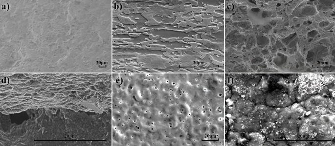
SEM images of various metal failure modes: (a) Metal fatigue; (b) Instantaneous stress-induced plastic deformation; (c) Stress corrosion cracking; (d) Thermal cycling; (e) Oxide deposition spalling; (f) Deposition-induced thermal corrosion.
Dataset
Data sources and classification scheme
The SEM image data used in this study were sourced from open-access materials science papers in the field of metal material preparation, performance testing, and failure analysis from the sci-hub repository. A total of 1,964 SEM images with explicit identification of metal failure were manually selected. Subsequently, based on the explanations provided in the papers for the SEM images and in conjunction with common classification schemes in the field of materials science for metal failure analysis, a two-level classification scheme was refined and annotated. The first level was used to identify the root causes of metal material failure, i.e. failure caused by mechanical forces or thermal effects. The second level was used to further subdivide each first-level category into three subcategories. The mechanical force induced-failure was further divided into three subcategories including metal fatigue, instantaneous stress-induced plastic deformation (such as tensile and compression), and stress corrosion cracking. The failure caused by thermal effects was further divided into thermal cycling, oxide deposition spalling, and deposition-induced thermal corrosion. Finally, the data were divided into the training set and testing set according to the ratio of 9:1. After processing, the specific data categories and distribution are listed in Table 1.
Theoretical basis of the data classification scheme
Metal fatigue is a material degradation process in which cyclic loading induces the initiation and propagation of microcracks, ultimately resulting in the occurrence of fracture (Fig. 1). Figure 1(a) presents the SEM image as an example of metal fatigue data. This is usually due to local stress exceeding the material limit at stress concentration sites (such as microcracks, pits, or scratches), leading to the gradual propagation of cracks. Long-term repeated stress (even below the strength limit of material) can also cause the dislocation movement and multiplication in the metal lattice to reduce the intergranular force, and eventually the fatigue cracks can be generated in the material.
Instantaneous stress causes permanent plastic deformation on a macroscopic level, while on a microscopic level this is caused by the movement and interaction of dislocations in the slip system41. When the stress exceeds the limit of fracture strength, the fracture occurs. The fracture modes can be divided into brittle fracture and ductile fracture. Figure 1(b) presents the SEM image for an example of permanent plastic deformation caused by mechanical force. Brittle fracture typically occurs suddenly without obvious prior indication of plastic deformation, which is predominantly driven by the rapid expansion of cracks. This type of fracture usually appears in materials with brittle crystal structures and a high density of defects (such as microcracks, voids, inclusions, etc.). Ductile fracture is always characterized by obvious plastic deformation prior to failure, as the material undergoes considerable deformation before fracture with gradual crack propagation.
The stress corrosion cracking (SCC) is a complex phenomenon that is primarily caused by the combined action of stress state and corrosive environment42. The tensile stress can be applied directly or may result from residual stress introduced during manufacturing processes such as cold working, welding, heat treatment, machining, and grinding. These residual stresses can significantly affect the susceptibility of materials to SCC. Additionally, SCC is closely associated with the specific combination of material, service environment, and stress conditions. Figure 1(c) shows SEM image for an example of stress corrosion cracking. It indicates that the formation and growth of cracks in a corrosive environment can lead to the unexpected and sudden failure of ductile metal alloys under tensile stress, especially at high temperatures. SCC exhibits a high degree of chemical specificity, as certain alloys are prone to SCC only when exposed to a limited number of specific chemical environments. Such chemical environments are often only mildly corrosive to the alloys, but SCC can be still induced. As a result, metal parts severely affected by SCC may appear shiny on the surface but are internally filled with micro-cracks. SCC typically progresses rapidly and is more prevalent in alloys than in pure metals. The specific environment is critical, and only very low concentrations of certain highly reactive chemicals are required to initiate catastrophic cracking, such as chloride ions or hydrogen sulfide, thereby leading to sudden and unexpected failure of critical components.
Thermal cycling refers to the process of repeatedly exposing a material to alternating high and low temperatures43. During this process, the temperature gradient and thermal stress are generated due to differences in the coefficients of thermal expansion among various components or layers. The thermal stress can lead to deformation, cracking, or other forms of material degradation. Figure 1(d) shows the SEM image for an example of thermal cycling data. As thermal cycling progresses, these thermal stresses can bring about the change of microstructure, such as the generation and movement of dislocations, and the migration of grain boundaries. Over time, these microcracks may coalesce and evolve into macroscopic cracks, ultimately compromising the structural integrity of material and leading to catastrophic failure. Failures caused by thermal cycling are common in fields such as turbine blades in aircraft engines and electronic packaging materials.
Oxide deposition spalling refers to the phenomenon where the formation of an oxide layer on the surface of metal materials at high temperatures can provide oxidation resistance, and then it undergoes cracking or detachment due to mechanical or thermal stress44. This protective oxide layer is initially dense and serves to prevent further oxidation of the underlying metal, whereas its integrity can be compromised by tensile stress that develops within the oxide layer, which is derived from differential thermal expansion between the oxide and the metal substrate. Additionally, external mechanical forces or repeated thermal cycling can induce spalling, leading to the exposure of the underlying metal and potentially accelerating further oxidation. Figure 1(e) shows the SEM image for an example of failure caused by oxide deposition and peeling. Once the protective oxide layer is compromised, the underlying metal undergoes rapid oxidation, significantly accelerating material degradation. The spalling of oxide layers can lead to the obstruction of critical precision components, such as engine oil passages, thereby impairing lubrication and potentially resulting in mechanical failure.
The deposition- induced thermal corrosion refers to the condition that impurities in fuels or lubricating oils, such as sodium, potassium, and vanadium, can deposit on the material surface at high temperature45. Figure 1(f) shows the SEM image for an example of the failure caused by the deposition- induced thermal corrosion. These deposits can chemically react with the material, destroying the protective oxide film on the material surface and exposing the substrate to a corrosive environment. The deposits may also form low-melting-point eutectics with the material, leading to localized melting and accelerating material failure. Thermal corrosion is widely present in high-temperature components such as aircraft engines and gas turbines.
The present classification scheme was designed on the basis of the following considerations. Firstly, the classification scheme included the two major types of metal material failure, i.e. failure caused by mechanical forces and failure caused by thermal effects. These two types of failure modes are widely present in engineering practice and have a significant impact on the service performance of materials. Secondly, under each main failure mode, it was subdivided into three subcategories, each corresponding to a specific failure mechanism. This classification method can be helpful to systematically and comprehensively understand the failure process of materials, and provides guidance for material selection, application and maintenance. Additionally, the proposed classification scheme is closely integrated with engineering practice, with each type of failure mode corresponding to specific engineering issues. For instance, fatigue failure is common in components subjected to cyclic loads, while thermal corrosion failure is common in components operating in high-temperature environments. This classification method can address the material failure issues in engineering in a targeted manner. Meanwhile, the cutting-edge research directions in the field of materials science are also involved in the present classification scheme. For example, the failure caused by thermal cycling is an important subject in aerospace and energy sectors, while oxide spalling, and thermal corrosion are hot topics in the field of high-temperature materials. This classification approach can provide a innovated perspective for understanding the latest advancements in the study of material failure dynamics.
Experimental methods
HFFNet_2D network architecture
As illustrated in Fig. 2, HFFNet_2D integrates CNN and Transformer architectures to perform hierarchical feature extraction and classification of metal failure images. In the implementation of the HFFNet_2D module, a pre-trained ResNet50 is first used as the backbone network for extracting local features from images. ResNet50 is a classic CNN structure that effectively alleviates the gradient vanishing problem in deep network training through residual connections, achieving efficient image feature extraction. Specifically, the pre-trained CNN ResNet50 was selected as the backbone network for feature extraction due to its well-established ability to capture hierarchical feature representations efficiently while maintaining computational feasibility. As compared to other CNN architectures, ResNet50 can provide deeper feature extraction capabilities while mitigating vanishing gradient issues through residual connections. By integrating ResNet50 with our Transformer encoder, its local feature extraction capabilities can be utilized while benefiting from the global context modeling of the Transformer. In this work, the first four convolutional blocks of ResNet50 were employed as a feature extractor, with the output feature map size being 1/32 of the original image size. After obtaining the adapted feature map, the HFFNet_2D module introduced learnable position encoding (pos_embedding). As an important component in the Transformer structure, position encoding was used to assign unique position information to each position in the feature map. By adding position encoding to the feature map, the model can consider the spatial relationships of features in subsequent self-attention calculations to better capture the global information of the image.

HFFNet 2D Network Architecture.
In addition to position encoding, the HFFNet_2D module also introduced a learnable class embedding vector (cls_token) as an additional input to the Transformer. The class embedding vector can be regarded as a global representation of the entire image, which can facilitate the model better understand the overall semantics of the image and capture relationships between different categories by interacting with local features. In the implementation, the class embedding vector was expanded to the same spatial dimension as the feature map and concatenated with the feature map along the channel dimension.
On the feature map that fused position encoding and class embedding, the HFFNet_2D module applied the Transformer2D submodule for further feature extraction and fusion. The Transformer2D submodule was composed of multiple self-attention layers and feed-forward neural networks, which can model long-range dependencies between different positions in the feature map, achieving efficient utilization of global image information.
After processing by the Transformer2D submodule, the HFFNet_2D module extracted the average of the class embedding vector and local features respectively and concatenated them along the channel dimension to form the final feature representation of the image (prim_rep). Finally, predictions for different levels of categories were made through multiple fully connected layers (level_fc) and classifiers (level_classifier). The fully connected layers mapped the final feature representation to feature spaces of different levels, while the classifiers performed classification predictions based on the mapped features.
Transformer2D module
The Transformer2D module was used to apply the self-attention mechanism on feature maps to model long-range dependencies between different regions. This module was composed of multiple stacked Transformer encoder layers, with each encoder layer containing two sub-modules: MultiHeadAttention2D and FeedForward2D. In each encoder layer, the multi-head self-attention mechanism first calculated the correlations between different feature positions to aggregate and interact global information. Subsequently, the feed-forward neural network performed nonlinear transformations on the aggregated features, enhancing the representational capacity of model. By stacking multiple encoder layers, deep-level extraction and fusion of image features can be achieved.
MultiHeadAttention2D submodule
As a key component of the Transformer2D module, the MultiHeadAttention2D submodule applied multi-head self-attention mechanism on feature maps to model long-range dependencies between different positions. In the implementation of the MultiHeadAttention2D submodule, the input feature map was first linearly transformed into query (Q), key (K), and value (V) tensors through 1 × 1 convolutional layers (qkv). The dimensions of these three tensors are (B, 3, num_heads, H, W, head_dim), where B is the batch size, num_heads is the number of attention heads, H and W are the spatial dimensions of the feature map, and head_dim is the dimension of each attention head. Subsequently, the MultiHeadAttention2D submodule splits the Q, K, V tensors into num_heads attention heads and performs self-attention calculations independently for each attention head. Specifically, for each attention head, the submodule first calculated the dot product between the query tensor Q and the key tensor K, and then was divided by the square root of head_dim to obtain attention scores. The attention scores were passed through a Softmax function to obtain attention weight. Finally, the attention weights were multiplied with the value tensor V and concatenated along the num_heads dimension to obtain the output feature map. To further enhance the representational capacity of features, the MultiHeadAttention2D submodule introduced an additional 1 × 1 convolutional layer (proj) to adjust the number of channels in the output feature map to match the input feature map. This step can be regarded as fusing features from different attention heads to obtain richer and more abstract representations. Through the multi-head self-attention mechanism, the MultiHeadAttention2D submodule can capture relationships between features at multiple scales and extract global information of images from multiple perspectives.
FeedForward2D submodule
As another component of the Transformer2D module, the FeedForward2D submodule was used to perform nonlinear transformations on the feature map output by the MultiHeadAttention2D submodule to further enhance the representational capacity of model. In the implementation of the FeedForward2D submodule, two 1 × 1 convolutional layers and a GELU activation function were used. The first convolutional layer (Conv2 d) expanded the number of channels in the input feature map from dim2 to hidden_dim, increasing the dimensionality of the features. After then, the GELU activation function was applied to introduce nonlinearity. Finally, the second convolutional layer (Conv2 d) can reduce the number of channels from hidden_dim back to dim2 to match the input dimension of subsequent layers. Through this structural design, the FeedForward2D submodule can perform multi-level nonlinear transformations on the feature map, extracting more abstract and high-level feature representations. Simultaneously, based on 1 × 1 convolutional layers, the FeedForward2D submodule can maintain the spatial dimensions of the feature map unchanged, ensuring that the position information of features is preserved.
Hierarchical feature fusion module
To effectively utilize the hierarchical structural information of images, the HFFNet model introduced a hierarchical feature fusion module. The input to this module was the output features from the Transformer encoder, including class embedding vectors and image patch embeddings. First, global average pooling was performed on the image patch embeddings to obtain a global feature vector. The global feature vector was concatenated with the class embedding vector to construct a comprehensive image representation. Subsequently, multiple fully connected layers were used to transform this comprehensive representation, generating feature representations at different levels. Each fully connected layer can be assigned to a specific level, learning semantic information at that level. Finally, the feature representations of different levels were concentrated to obtain the fused feature vector as the final representation of the image.
Classification output
After obtaining the fused image feature representation, the HFFNet model used multiple classifiers to perform hierarchical classification of the image. Each classifier was a fully connected layer corresponding to a specific level. The input to the classifier was the fused image feature, and the output is the category probability distribution at that level. Through the collaborative work of multiple classifiers, the HFFNet model can simultaneously predict category labels at different levels for the image. During training, the cross-entropy loss function was used to supervise the classification results at each level, and the losses of all levels were added up as the final optimization objective. This multi-task learning approach can make the model better utilize the correlations between different levels and improve overall classification performance.
Adjustable parameters of the network
The HFFNet-2 d network incorporated several key adjustable parameters that can significantly influence its performance and structure. The input image size (img_size) determined the dimensions of the data fed into the network. For the hierarchical metal failure analysis task, the number of categories (num_classes) was set to2,7, representing two categories at the first level and six at the second level. The Transformer’s feature dimension (dim) was crucial as it defined the input and output dimensions for both the self-attention mechanism and the feed-forward neural network within the Transformer. The depth parameter, which specified the number of Transformer encoder layers, allowed for deeper feature extraction and fusion, albeit at the cost of increased computational complexity. In the multi-head self-attention mechanism, the number of heads (heads) enabled the model to learn richer feature representations from various subspaces. Eventually, the hidden layer dimension of the Transformer’s feed-forward neural network (mlp_dim) was increased to improve the representational capacity of the network, although it also led to an increase in the overall number of model parameters.
Data preprocessing and model training
Data preprocessing
To enhance the generalization ability and robustness of model, various data preprocessing techniques were adopted. For the training set, the data augmentation methods were implemented, including Random Resized Crop, Random Horizontal Flip, Random Rotation, Normalization, and Random Erasing. Data augmentation techniques used in our study, including Random Resized Crop and Random Horizontal Flip, were carefully selected based on our understanding of SEM image characteristics and validated through experiments. These methods can effectively preserve critical microstructural features of material failure regions while improving model robustness. Unlike augmentations that might distort physical interpretations (such as vertical flipping or extreme color alterations), the selected techniques can maintain the scientific validity of failure mechanisms—Random Resized Crop preserves key morphological features like cracks and fatigue striations, while Random Horizontal Flip respects the topological relationships since the material failures exhibit similar characteristics regardless of orientation. All augmentation strategies were verified by materials science experts to ensure they maintained the physical significance and recognizability of microstructural features, ultimately enhancing model generalization without compromising the scientific integrity of the SEM imagery.
Optimization algorithm and loss function
Stochastic Gradient Descent (SGD) was selected as the optimization algorithm, with an initial learning rate of 1e-4, momentum of 0.937, and weight decay of 5e-4. These parameters were selected to accelerate convergence, reduce oscillations, and prevent overfitting. The loss function design combined Focal Loss and Label Smoothing techniques. The total training loss was calculated as a weighted sum of losses from two branches, with the second branch given higher weight to reflect its importance in hierarchical classification. The loss functions for each branch are defined as follows:
where \(\:\alpha\:\) is the balancing factor, \(\:\gamma\:\) is the focusing parameter, \(\:{p}_{1}\) and \(\:{p}_{2}\) represent the prediction probabilities of model for the true categories in each branch, \(\:{q}_{1i}\) and \(\:{q}_{2i}\) represent the smoothed true probability distributions, and \(\:{\widehat{y}}_{1i}\) and \(\:{\widehat{y}}_{2i}\) represent the model’s prediction probabilities for each category in the respective branches.
Training hyperparameters
The training process utilized a batch size of 16, balancing training efficiency and memory consumption. We trained the model for 200 epochs to ensure sufficient convergence. A Cosine Annealing (CosineAnnealingLR) learning rate scheduling strategy was employed to dynamically adjust the learning rate during training, adapting to optimization needs throughout the process. In our final model, a 12-layer Transformer depth with 12 attention heads was employed, with the model dimension set to 768 and the MLP dimension set to 3072. The input image size was (224, 224). All other parameters remained consistent throughout the ablation experiments.
Evaluation metrics
Hierarchical Precision (HP) measures the proportion of true positives among the samples predicted as positive by the model. HP can be expressed by the following formula:
where \(\:{T}_{i}\) represents the set of true categories for the i-th sample, \(\:{P}_{i}\) represents the set of predicted categories for the i-th sample.
Hierarchical Recall (HR) measures the proportion of correctly predicted samples among the samples with true positive labels. HR can be expressed by the following formula:
Hierarchical F-score (HF) is the weighted harmonic mean of HP and HR, comprehensively considering precision and recall, providing a more comprehensive evaluation of model performance in hierarchical multi-label classification tasks. HF can be expressed by the following formula:
where \(\:\beta\:\) is a parameter adjusting the weights of HP and HR. Typically, \(\:\beta\:\) is set to 1, indicating that HP and HR are equally important. In this case, HF degenerates to HF1, and the calculation formula can be simplified as follows:
Ablation experiments and algorithm analysis
To validate the effectiveness of the HFFNet-2 d network’s module design and explore the impact of different architectures on model performance, we conducted a series of ablation experiments. Four variant models were designed: HFFCNN, HFFVT, HFF_CNN_VT, and HFF_CNN_Conv_VT. By comparing these variants with HFFNet-2 d, it aims to better understand its advantages and limitations.
HFFVT model
The baseline version, HFFVT, was constructed based on the original ViT structure. It directly divided the input image into fixed-size patches and used linear projection for Transformer input. Unlike HFFNet-2 d, HFFVT cannot use CNN for feature extraction, potentially reducing parameters and computational complexity. However, this design may not fully utilize local features and semantic information. The direct addition of position encoding to image patch embeddings, without considering CNN feature spatial structure, may impact the ability to model spatial information.
HFFCNN model
The HFFCNN model extended the baseline concept using a convolutional neural network (ResNet50) for feature extraction while suppressing the HFF module and HFFVT. This model served as a direct comparison with HFFVT to explore performance differences between transformer and CNN structures.
HFF_CNN_VT model
HFF_CNN_VT combined convolutional neural networks and transformers. It used the first four convolutional blocks of ResNet50 for feature extraction before transforming these features into Transformer input. Compared to HFFNet-2 d, it used linear projection instead of convolutional layers for feature mapping, potentially reducing parameters but possibly underutilizing spatial structure information. The position encoding size matched the number of image patches, which may affect the ability of model to capture spatial information effectively.
HFF_CNN_Conv_VT model
Building on HFF_CNN_VT, the HFF_CNN_Conv_VT model replaced linear projection with a 1 × 1 convolutional layer to transform CNN features into Transformer input. However, similar to HFF_CNN_VT, its position encoding size matched the image patch number and is directly added to the Transformer input without considering CNN feature spatial structure. This approach may impact the model’s spatial information modeling capabilities. All the ablation experiments were maintained consistent network hyperparameters and training parameters with HFFNet-2 d to ensure experimental validity.
Results
Model results
As illustrated in Fig. 3, three graphs exhibit the training process: the loss curve (left), the accuracy curve for Level 1 (center), and the accuracy curve for Level 2 (right). In each graph, the blue line represents metrics from the training set, while the red line indicates corresponding metrics from the test set. The proposed HFFNet-2 d network can achieve excellent performance on the metal failure analysis task, outperforming other ablation experiment networks on all evaluation metrics. As shown in Table 2, HFFNet-2 d achieves 0.9587, 0.9690, and 0.9639 in terms of hP, hR, and hF1, respectively. These results demonstrate the effectiveness of the HFFNet-2 d architecture in solving hierarchical multi-label classification problems. Moreover, HFFNet-2 d achieves the best results in Level-1 and Level-2 accuracies, reaching 97.93% and 92.75%, respectively, indicating its ability to accurately identify metal failure modes at different granularities. Compared to HFFVT, HFFNet-2 d can improve Level-1 Acc by 6.09% and Level-2 Acc by 11.37%.

Accuracy vs. loss curve of HFFNet 2D.
By comparing the performance of different ablation experiment networks, we can gain a deeper understanding of the design advantages of HFFNet-2 d. The basic version HFFVT is clearly inferior to other networks on all metrics, indicating that using only the Transformer structure cannot fully utilize the local features and semantic information of SEM images. After introducing CNN for feature extraction, HFF_CNN_VT’s performance is significantly improved, but there is still room for improvement in Level-2 accuracy. HFF_CNN_Conv_VT can further enhance the classification performance using convolutional layers instead of linear projections to transform CNN features into Transformer input. However, it shows a slight decrease in Level-2 accuracy, possibly due to the lack of position encoding, resulting in partial loss of spatial information.
HFFNet-2 d can optimize and improve upon the above networks by using convolutional layers to transform CNN features into Transformer input and introducing position encoding with the same spatial dimensions as the CNN feature maps. This design fully utilizes the spatial structure information of CNN features while avoiding conflicts between position information and feature information. The experimental results show that this design enables HFFNet-2 d to achieve the best performance in hierarchical multi-label classification tasks, especially with significant improvements in Level-2 subclass identification.
As shown in Figs. 4 and 5, the confusion matrices for both classification levels demonstrate excellent model performance in the two-level classification task, particularly achieving high accuracy (97.9%) at Level-1 classification. The confusion matrix shows 79 correct predictions for mechanical force-induced failures with only 2 misclassifications, and 110 correct predictions for thermal effect-induced failures with merely 2 misclassifications. Level-2 classification also performs well (92.7% accuracy), with thermal cycling showing the best recognition results (67/72 correct). Stress corrosion cracking, oxide deposition spalling, and deposition-induced thermal corrosion can achieve the accuracy rates of 92.3%, 90.0%, and 95.0% respectively. Metal fatigue and instantaneous stress-induced plastic deformation reaches the accuracy rates of 93.8% and 91.7%, respectively. Overall, both levels of classifiers demonstrate strong generalization capabilities and classification accuracy.

Level 1 confusion matrices of HFFNet 2D.

Level 2 confusion matrices of HFFNet 2D.
Model visualization and interpretability analysis using Grad-CAM technique
The Grad-CAM algorithm was adopted to perform model visualization and interpretability analysis on the trained HFFNet_2D. Grad-CAM (Gradient-weighted Class Activation Mapping) was used to explain the decisions of convolutional neural networks (CNNs). The heat maps were obtained to visualize the image regions that the model focuses on when making predictions, which can provide an in-depth understanding of the decision-making process of CNN models.
The principle of Grad-CAM used the gradient information to determine the importance of each position in the image for the model to make specific predictions. The gradients of the predicted class with respect to the feature maps of the last convolutional layer were calculated, and the weights of each feature map were obtained through global average pooling of the gradients. These weights were then multiplied by the corresponding feature maps and summed to generate the class activation heat map. Eventually, the heat map was upsampled and overlaid on the original image to visualize the regions of focus for the model. Since the algorithm operated at two levels, the regions of interest for the model were identified at both category levels. Several heat maps were selected for display.
In the original SEM image (Fig. 6), typical fatigue features such as river-like fatigue striations or beach marks can be detected. These features are related to changes in stress intensity factor and cyclic stress, serving as evidence of fatigue crack propagation. In the task1 CAM heatmap, the neural network shows particular attention to certain hotspot areas on the fracture surface. These areas represent important features along the crack initiation point and crack propagation path. Such features include rough fracture surfaces, microcracks, or crack branching points, all of which are critical in the fatigue fracture process. In the task 2 CAM, the points of focus are more dispersed, concentrating on different parts of the fracture surface. This may be because the task emphasizes different features, such as fine microcracks, plastic deformation zones, or changes in the material’s internal microstructure.

Heatmaps of HFFNet-2 d on metal fatigue.
As shown in Fig. 7, the SEM image exhibits a large number of dimples, which are formed when plastic deformation occurs in areas of local stress concentration in the material. This structural feature typically indicates that the material underwent significant plastic deformation before fracture, which is a characteristic of ductile fracture. In the task1 CAM heatmap, the high-attention areas in red and orange are concentrated on specific dimples. The neural network likely identifies these areas because the shape, size, or distribution characteristics of these dimples are closely related to ductile fracture features. For instance, larger dimples usually indicate greater plastic deformation, which might be the focus of the network’s attention. Similarly, large and deep dimples typically suggest that the material has undergone substantial plastic deformation, which is an important feature in fracture analysis. The heatmap for Task2 CAM shows more dispersed attention areas, covering a broader range of dimple regions. This may indicate that the model for task 2, when identifying microscopic features of the fracture, focuses on the overall dimple structure and surface microdetails, as well as the fine structures within the dimples, such as bridging between dimples and the presence of microcracks. These features may help the model distinguish between different types of fracture modes or material characteristics, as well as the fracture history.

Heatmaps of HFFNet-2 d on dimples.
As illustrated in Fig. 8, it reveals a distinct crack path and surrounding fracture features. The crack initiates from the upper left corner and extends downward to the lower middle part of the image, exhibiting a typical fatigue fracture pattern. This fracture is likely caused by cyclic stress, leading to gradual crack formation and ultimately resulting in failure.

Heatmaps of HFFNet-2 d on fracture features.
Task 1 CAM: The heatmap shows high attention areas in red and yellow around the crack initiation point and along the crack path. These areas typically represent the crack initiation point and stress concentration zones. In particular, the red highlight at the crack initiation point indicates a significant fracture feature. This is typically where stress concentration is most pronounced, often resulting from microstructural defects or material inhomogeneities that facilitate crack initiation. Alternatively, it may be attributed to microscopic flaws or other factors that act as stress concentrators, leading to the occurrence of failure.
Task 2 CAM: The heatmap shows attention areas extending to more regions along the crack path and its surroundings. This might be because the model for Task 2, when identifying fracture features, not only considers the crack initiation point but also focuses on the crack propagation path. The highlighted areas may reflect changes in the material’s microstructure, such as grain boundary sliding or microcrack propagation.
As shown in Fig. 9, the structural features on and near the material surface indicate that the material has undergone oxidation and thermal degradation processes in a high-temperature environment. The structures depicted in the image may encompass oxide deposition layers and oxide spallation phenomena resulting from thermal stress. The brighter areas at the top of the image are likely oxide deposition layers. When the materials are exposed to high-temperature environments, their surfaces react with oxygen to form oxides. These oxide layers can be either protective or detrimental, depending on the material and its usage environment. The structure beneath the oxide layer shows some irregular morphology, which may be due to oxide spallation caused by thermal stress. Spallation typically occurs due to differences in thermal expansion coefficients between the material surface and the oxide layer, leading to stress concentration and interfacial delamination.

Heatmaps of HFFNet-2 d on oxidation and thermal damage.
In Task 1 CAM, the neural network shows high attention to specific areas. These areas are likely thicker parts of oxide deposits or crack initiation points. Cracks and spallation usually occur at the interface between the oxide layer and the substrate material. The high attention to these areas in the heatmap may be because these features are precursors to material failure. The network might use these features to identify abnormalities or damage on the material surface.
Discussion
Impact of data collection and classification scheme
A key challenge in the metal failure analysis task is to obtain a sufficient quantity and quality of SEM image data. In this study, 1,964 SEM images were obtained from open-access materials science papers, which to some extent limited the scale and diversity of the dataset. The size and quality of the dataset directly affect the performance of deep learning models, especially in fine-grained classification tasks at the second level. Different failure modes may have similarities and overlaps in morphology and features in SEM images, making it difficult for the model to accurately distinguish them. Furthermore, there may be issues with the annotation quality and consistency of the dataset. Different experts may have different judgments and annotations for the same SEM image, introducing noisy data that negatively impacts the model’s learning and generalization abilities. Additionally, class imbalance in the dataset may be a factor. For example, if the number of samples in the hot corrosion category is relatively small, the model’s ability to learn and recognize this category may be weak, leading to bias towards categories with more samples.
To further improve the performance of HFFNet-2 d in metal failure analysis tasks, we can improve the data collection and classification scheme from multiple aspects. First, optimizing the annotation quality and consistency of the dataset is crucial. This can be achieved through cross-annotation and review by multiple ___domain experts, as well as data cleaning and filtering steps to improve the accuracy and consistency of the dataset. Additionally, refining the classification scheme and label system is a direction worth exploring. Based on ___domain knowledge and expert feedback, we can introduce more fine-grained failure mode subclasses, as well as multi-level or multi-branch label systems, to more accurately and comprehensively describe the influencing factors of metal failure. It also should be noted that the quality and variability of the SEM images used for training and testing our model can significantly impact prediction accuracy. Factors such as image resolution, contrast, and noise levels can introduce errors. Besides, the inherent variability in metal failure patterns across different samples can pose challenges in achieving high accuracy. For the mitigation strategies, the advanced data preprocessing techniques can be implemented to enhance image quality, including noise reduction, contrast adjustment and normalization. Furthermore, despite the encouraging results achieved by the HFFNet-2 d model in metal failure classification, several challenges remain unresolved. The current dataset is limited to only 1,964 images with significant class imbalance, and 727 thermal cycling samples are involved, but the number of stress corrosion cracking samples is merely 137, substantially limiting the recognition capabilities of this model for rare failure modes. Additionally, the model performs inadequately when handling composite failure scenarios involving multiple concurrent failure mechanisms, which are common in real engineering applications. While Grad-CAM analysis was implemented, the model’s ability to distinguish between certain failure types with similar surface morphological features still needs further improvement. Meanwhile, the current model lacks cross-___domain generalization capability for unseen material systems, restricting its effective application to SEM images acquired from different laboratories or equipment.
To address these challenges, several potential solutions are proposed. Targeted supplementation of additional data for underrepresented classes would help address the data imbalance issue. Incorporating metadata such as material composition, processing history, and service conditions as auxiliary information could build multimodal learning frameworks that enhance the model’s ability to differentiate between failure types with similar morphologies. Implementation of transfer learning and ___domain adaptation techniques would enhance the model generalization across different material systems and experimental equipment. Development of knowledge-based neural network architectures that integrate expert knowledge with physical models and materials science principles would ensure predictions conform to physical and materials science laws, further enhancing the practicality and reliability of automated metal failure analysis systems for engineering applications.
Exploring applications of the HFFNet-2 d architecture in other materials science domains
The HFFNet-2 d network architecture has demonstrated excellent performance in metal failure analysis tasks. Its design concept of integrating CNN and Transformer, as well as its capability to handle hierarchical multi-label classification problems, shows broad application prospects. In the next phase, we plan to extend the HFFNet-2 d network architecture to other areas of materials science, such as material defect detection, microstructure classification, and material property prediction. In the field of material defect detection, the HFFNet-2 d network can be utilized to identify and localize various defects in material samples (e.g., metals, ceramics, composites), such as pores, cracks, and inclusions. By adopting a multi-task learning approach and combining the classification results of HFFNet-2 d with object detection algorithms (e.g., Faster R-CNN and YOLO), automatic localization and segmentation of defects can be achieved, improving the efficiency and accuracy of defect detection. This has significant implications for quality control and process optimization.
For materials microstructure classification, the HFFNet-2 d network can be employed to recognize and classify microstructural features of materials (e.g., metals, rocks, biomaterials), including grain morphology, precipitate distribution, and pore structure. By introducing multi-scale feature extraction and attention mechanisms, the HFFNet-2 d network can capture multi-scale features and key regions of material microstructures, enabling more refined and comprehensive microstructure characterization. This is valuable for understanding the microstructure-property relationships of materials and optimizing material processing parameters. In the ___domain of material property prediction, the HFFNet-2 d network can be used to establish mapping relationships between material microstructures and properties, enabling material property prediction based on microstructure images. By combining the feature extraction module of HFFNet-2 d with regression models (e.g., support vector machines and neural networks), mechanical properties, physical properties, and functional characteristics of materials can be predicted from their microstructure images. This approach can significantly reduce the time and cost of material property testing, accelerating material development and screening. The HFFNet-2 d network can provide a powerful and effective tool for image analysis and intelligent decision-making in materials science. Future work can further explore the extension and optimization of the HFFNet-2 d network in different material systems and application scenarios, and integrate it with expert knowledge and experimental techniques in the materials field. This will establish a new paradigm for intelligent analysis and decision-making in materials science, promoting innovation and development in the field.
Conclusion
In this study, a hierarchical multi-label classification method called HFFNet-2 d is proposed for automated classification of scanning electron microscope (SEM) images in engineering metal failure analysis. HFFNet-2 d ingeniously combines the advantages of convolutional neural networks (CNN) and visual Transformers (ViT), introducing ResNet50 as the backbone network for local feature extraction and employing a Transformer encoder to model global dependencies, and thereby hierarchical feature extraction and classification of SEM images are achieved. In metal failure analysis tasks, HFFNet-2 d demonstrates exceptional performance, surpassing other comparative models in all evaluation metrics, proving its effectiveness in handling complex hierarchical multi-label classification problems. Notably, HFFNet-2 d can achieve a high accuracy of 97.71% in first-level classification (stress failure vs. thermal treatment failure) and 92.62% accuracy in second-level subclass identification, indicating its ability to accurately grasp both the macroscopic causes of material failure and specific failure mechanisms. These results demonstrate the outstanding performance HFFNet-2 d in solving hierarchical multi-label classification tasks for SEM images. It can further expand the optimization and application of HFFNet-2 d in different material systems and application scenarios, accelerating the intelligent process of material development and failure analysis, which probably provides strong support for ensuring the safety of engineering structures and improving the efficiency of material design.
Data availability
Data will be made available on reasonable request. Please contact the corresponding author Haoran Zheng ([email protected]) to get the datasets and source code.
References
Zimmermann, N. & Wang, P. H. A review of failure modes and fracture analysis of aircraft composite materials. Eng. Fail. Anal. 115, 104692 (2020).
Panwar, A. S., Singh, A. & Sehgal, S. Material characterization techniques in engineering applications: A review. Mater. Today: Proc. 28, 1932–1937 (2020).
Wang, L., Yang, L. J., Wang, L. Y., Tang, X. J. & Liu, G. Influence mechanism of grinding surface quality of 20CrMnTi steel on contact failure. Sci. Rep. 14, 13374 (2024).
Pineau, A., Benzerga, A. A. & Pardoen, T. Failure of metals I: brittle and ductile fracture. Acta Mater. 107, 424–483 (2016).
Tomota, Y., Xia, Y. & Inoue, K. Mechanism of low temperature brittle fracture in high nitrogen bearing austenitic steels. Acta Mater. 46, 1577–1587 (1998).
Salvati, E. Evaluating fatigue onset in metallic materials: problem, current focus and future perspectives. International J. Fatigue 108487 (2024).
Kumar, V., Pujari, A. K., Padmanabhan, V., Sahu, S. K. & Kagita, V. R. Multi-label classification using hierarchical embedding. Expert Syst. Appl. 91, 263–269 (2018).
Vens, C., Struyf, J., Schietgat, L. & Džeroski, S. Blockeel. Decision trees for hierarchical multi-label classification. Mach. Learn. 73, 185–214 (2008).
Huang, W. et al. HmcNet: A general approach for hierarchical Multi-Label classification. IEEE Trans. Knowl. Data Eng. 35, 8713–8728 (2022).
Li, Q. et al. A survey on text classification: from traditional to deep learning. ACM Trans. Intell. Syst. Technol. (TIST). 13, 1–41 (2022).
Feng, S., Zhao, C. & Fu, P. A deep neural network based hierarchical multi-label classification method. Rev. Sci. Instrum. 91, 2 (2020).
Gargiulo, F., Silvestri, S., Ciampi, M. & De Pietro, G. Deep neural network for hierarchical extreme multi-label text classification. Appl. Soft Comput. 79, 125–138 (2019).
LeCun, Y., Bengio, Y. & Hinton, G. Deep Learn. Nature 521, 436–444 (2015).
Yang, D. et al. Detection and analysis of COVID-19 in medical images using deep learning techniques. Sci. Rep. 11, 19638 (2021).
Wolf, D. et al. Self-supervised pre-training with contrastive and masked autoencoder methods for dealing with small datasets in deep learning for medical imaging. Sci. Rep. 13, 20260 (2023).
Kumar, Y. et al. Enhancing parasitic organism detection in microscopy images through deep learning and fine-tuned optimizer. Sci. Rep. 14, 5753 (2024).
Adibnia, E. et al. A deep learning method for empirical spectral prediction and inverse design of all-optical nonlinear plasmonic ring resonator switches. Sci. Rep. 14, 5787 (2024).
Calik, N. et al. Deep-learning-based precise characterization of microwave transistors using fully-automated regression surrogates. Sci. Rep. 13, 1445 (2023).
Krizhevsky, A., Sutskever, I. & Hinton, G. E. ImageNet classification with deep convolutional neural networks. Commun. ACM. 60, 84–90 (2017).
Archana, R. & Jeevaraj, P. S. E. Deep learning models for digital image processing: a review. Artif. Intell. Rev. 57, 11 (2024).
Oyedeji, O. A., Khan, S. & Erkoyuncu, J. A. Application of CNN for multiple phase corrosion identification and region detection. Appl. Soft Comput. 164, 112008 (2024).
Nimma, D. & Uddagiri, A. Advancements in deep learning architectures for image recognition and semantic segmentation. International J. Adv. Comput. Sci. & Applications 15, (2024).
Jaffari, Z. H. et al. Transformer-based deep learning models for adsorption capacity prediction of heavy metal ions toward biochar-based adsorbents. J. Hazard. Mater. 462, 132773 (2024).
Santiago, C., Carlos, M., Javier, C., Pascual, C. & Fernando, C. Natural Language processing: an overview of models, Transformers and applied practices. Comput. Sci. Inform. Syst. 00, 31 (2024).
Chen, C. et al. A survey on graph neural networks and graph Transformers in computer vision: A Task-Oriented perspective. IEEE Trans. Pattern Anal. Mach. Intell. https://doi.org/10.1109/TPAMI.2024.3445463 (2024).
Pradhan, P. K. et al. Swin sight: a hierarchical vision transformer using shifted windows to leverage aerial image classification. Multimedia Tools Applications 1–22 (2024).
Carion, N. et al. End-to-end object detection with transformers. European conference on computer vision. Cham: Springer International Publishing, (2020). https://doi.org/10.1007/978-3-030-58452-8_13
Zheng, H., Wei, S., Yu, W. & Young, B. Multi-label classification for metal defects from SEM images using deep learning. 2022 28th Int. Conf. Mechatronics Mach. Vis. Pract. (M2VIP). IEEE (1–6). https://doi.org/10.1109/M2VIP55626.2022.10041065 (2022).
Beniwal, A., Dadhich, R. & Alankar, A. Deep learning based predictive modeling for structure-property linkages. Materialia 8, 100435 (2019).
Yang, Z. et al. Establishing structure-property localization linkages for elastic deformation of three-dimensional high contrast composites using deep learning approaches. Acta Mater. 166, 335–345 (2019).
Azqadan, E., Jahed, H. & Arami, A. Predictive microstructure image generation using denoising diffusion probabilistic models. Acta Mater. 261, 119406 (2023).
de Haan, K., Ballard, Z. S., Rivenson, Y., Wu, Y. & Ozcan, A. Resolution enhancement in scanning electron microscopy using deep learning. Sci. Rep. 9, 12050 (2019).
Aversa, R., Coronica, P. & De Nobili, C. Cozzini. Deep learning, feature learning, and clustering analysis for Sem image classification. Data Intell. 2, 513–528 (2020).
Liang, Y. et al. Ultrahigh-resolution reconstruction of shale digital rocks from FIB-SEM images using deep learning. SPE J. 29, 1434–1450 (2024).
Sun, M., Niu, J., Yang, X., Gu, Y. & Zhang, W. CEHMR: curriculum learning enhanced hierarchical multi-label classification for medication recommendation. Artif. Intell. Med. 143, 102613 (2023).
Romero, M., Nakano, F. K., Finke, J., Rocha, C. & Vens, C. Leveraging class hierarchy for detecting missing annotations on hierarchical multi-label classification. Comput. Biol. Med. 152, 106423 (2023).
Noor, K. T. & Robles-Kelly, A. H-CapsNet: A capsule network for hierarchical image classification. Pattern Recogn. 147, 110135 (2024).
Dong, S. et al. Lightweight multi-scale encoder–decoder network with locally enhanced attention mechanism for concrete crack segmentation. Meas. Sci. Technol. 36, 025021 (2025).
Bogatinovski, J., Todorovski, L., Džeroski, S. & Kocev, D. Comprehensive comparative study of multi-label classification methods. Expert Syst. Appl. 203, 117215 (2022).
Krizhevsky, A. & Hinton, G. Learning multiple layers of features from tiny images, 7, (2009). https://www.cs.toronto.edu/kriz/learning-features-2009-TR.pdf
Ramazani, A., Schwedt, A., Aretz, A., Prahl, U. & Bleck, W. Characterization and modelling of failure initiation in DP steel. Comput. Mater. Sci. 75, 35–44 (2013).
Contreras, A., Hernández, S., Orozco-Cruz, R. & Galvan-Martínez, R. Mechanical and environmental effects on stress corrosion cracking of low carbon pipeline steel in a soil solution. Mater. Design. 35, 281–289 (2012).
Barako, M., Park, W., Marconnet, A., Asheghi, M. & Goodson, K. Thermal cycling, mechanical degradation, and the effective figure of merit of a thermoelectric module. J. Electron. Mater. 42, 372–381 (2013).
Zou, Y. et al. In-situ SEM analysis of brittle plasma electrolytic oxidation coating bonded to plastic aluminum substrate: microstructure and fracture behaviors. Mater. Charact. 156, 109851 (2019).
Yu, C., Zhu, S., Wei, D. & Wang, F. Oxidation and H2O/NaCl-induced corrosion behavior of sputtered Ni–Si coatings on Ti6Al4V at 600–650° C. Surf. Coat. Technol. 201, 7530–7537 (2007).
Acknowledgements
The presented investigations have been supported by the National Natural Science Foundation of China (No. 52401140).
Author information
Authors and Affiliations
Contributions
Ruitong Han was responsible for algorithm design, code development, and writing the original draft of the algorithm section of the paper. Chang-Bo Liu was responsible for defining the classification patterns, data analysis related to materials science, and writing the original draft of the results analysis. Wanting Sun provided guidance on the materials section and data analysis. Haoran Zheng provided guidance on algorithm establishment and design of comparative experiments. Shuai Yu and Lin Deng were responsible for data collection and screening. The original draft of the manuscript was written by Ruitong Han, and all authors commented on previous versions of the manuscript. All authors read and approved of the final manuscript.
Corresponding authors
Ethics declarations
Competing interests
The authors declare no competing interests.
Additional information
Publisher’s note
Springer Nature remains neutral with regard to jurisdictional claims in published maps and institutional affiliations.
Rights and permissions
Open Access This article is licensed under a Creative Commons Attribution-NonCommercial-NoDerivatives 4.0 International License, which permits any non-commercial use, sharing, distribution and reproduction in any medium or format, as long as you give appropriate credit to the original author(s) and the source, provide a link to the Creative Commons licence, and indicate if you modified the licensed material. You do not have permission under this licence to share adapted material derived from this article or parts of it. The images or other third party material in this article are included in the article’s Creative Commons licence, unless indicated otherwise in a credit line to the material. If material is not included in the article’s Creative Commons licence and your intended use is not permitted by statutory regulation or exceeds the permitted use, you will need to obtain permission directly from the copyright holder. To view a copy of this licence, visit http://creativecommons.org/licenses/by-nc-nd/4.0/.
About this article

Cite this article
Han, R., Liu, CB., Sun, W. et al. Machine learning of automatic hierarchical multi-label classification method for identifying metal failure mechanisms. Sci Rep 15, 19904 (2025). https://doi.org/10.1038/s41598-025-05076-z
Received:
Accepted:
Published:
DOI: https://doi.org/10.1038/s41598-025-05076-z
