
Abstract
Living organisms are frequently used as sentinels to monitor changes in the environment, and organoids can serve a similar function as in vitro sentinels detecting microbiological processes. One such process of great interest is pathogenic infection, which causes alterations in the cellular dynamics of the sentinels. Doppler light scattering is well suited to measure such changes, as it is sensitive to the intracellular dynamics of the organoids even when the microbe density is too dilute to detect directly. In this paper, we present measurements of the endogenous changes of intracellular dynamics of DLD organoids (microclusters) in response to bacterial infection, detected using a long-coherence form of biodynamic imaging (BDI), a dynamic-contrast digital holography technique that captures the Doppler shifts encoded in the dynamic speckles. With a stable common-path digital holography system and using small in-vitro tissue microclusters, clinically relevant inoculum doses as low as 100 cfu/mL cause detectable changes in intracellular Doppler spectra within hours of infection and several hours before the proliferating bacteria population causes direct light scattering. Because it can measure effects for small bacterial populations, the method shows promise as a fast diagnostic tool to detect the presence of bacteria in patient fluid samples faster than traditional methods.
Introduction
Bacterial infections remain a significant health concern globally, including in the developed world1. About 13.7 million people died from causes related to bacteria infection in 20192, and more than 11 million deaths worldwide and 270,000 deaths in the United States in 2020 are attributed to bacterial infection3. Efforts to curb the death toll with antibiotics is hampered by the proliferation of antibiotic-resistant bacteria4, which is exacerbated due to poor treatment management practices and indiscriminate use of antibiotics in the livestock industry5,6. It is projected that by 2050, antimicrobial resistance will incur a higher death toll than will cancer7.
Another factor that poses a significant challenge to the treatment of bacteria infection is the time dependence of the mortality rate from sepsis8, as identification of a bacterial strain and its susceptibility to antibiotics can be a time-consuming process. The standard clinical tests for antibiotic resistance, such as the disk diffusion method or the dilution method, require multiple iterations of bacteria culture to prepare the stock and identify the strain9, which takes up to 26 hours10. Even when the inoculum is not incubated to the full McFarland 0.5 standard, the time taken to perform the disk diffusion method itself means that the whole process still takes up to or over a day11. Meanwhile, a delay to effective treatment by just 48 hours can cause the mortality to jump from 10% to 40%12. Therefore, novel techniques capable of detecting the presence of bacteria, and their response to different antibiotics, on the timescale of hours rather than of days, are urgently needed.
Imaging techniques such as static and dynamic fluorescence microscopy can detect the number of bacteria present in host tissue by measuring the intensity of the light originating from known fluorescent tags13, and these methods can detect the presence of bacteria on short timescales on the order of a few hours. However, these techniques rely on fluorescence from engineered strains of known bacteria or the addition of fluorophores. Moreover, fluorescent imaging is often susceptible to signal-to-noise ratio degredation caused by photobleaching14. These constraints raise concerns about the techniques’ applicability when there is a need to detect a wild phenotype of an unidentified bacteria in clinical settings with minimal preparation under strict time constraints.
More recently, antimicrobial susceptibility testing (AST) techniques that leverage Raman spectroscopy have shown promise as a family of techniques that rapidly identify bacterial resistance to antibiotics15,16, but these methods still require the bacteria with which the patient is infected to be isolated and cultured, adding time to prepare the observation. A rapid testing method should jettison this requirement to achieve low detection limits with screening times on the order of hours.
Here we tackle this problem by leveraging a long-coherence, common-path mode of biodynamic imaging. This variant is a full-field dynamic-contrast imaging technique that maximizes sensitivity to dynamic speckle. The technique generates 2D projection of a thin tissue sample using off-axis holography. The diffusely scattered light from the tissue carries Doppler shifts caused by intracellular motions, and the partial-wave sums of the Doppler shifted light create dynamic speckle. The intensity fluctuations from the dynamic speckle can be used as a surrogate observable to study the distribution of intracellular dynamics and to track subtle changes over long timescales, visualized as differential spectrograms that are similar to the conventional definition of spectrograms in audio processing, but with the baseline spectrum subtracted to focus on the change of signal17. The idea of measuring the Doppler shift to measure dynamics is similar to that seen in, for instance, Doppler OCT angiography using18,19. However, the distinction is that in conventional dynamic OCT setup, the typical measurement of Doppler shift comes from macroscopic flow that is very far in the ballistic regime, whereas the measurement of intracellular motion lies in the middle between pure diffusion and pure ballistic motion17, with Doppler number on the order of 1\(\sim\)10.
Intracellular functions, and therefore dynamics, are disrupted by the presence of bacteria, resulting in changes in the fluctuation spectrum. Therefore, the technique detects bacterial infection by tracking the changes in the spectrum of intensity fluctuation in light scattered off of the host cells. The host cells serve as living biosensors; these organoid ‘sentinels’ stand watch for pathogens, emitting dynamic signals upon infection. To differentiate between infected and uninfected tissues, we simply observe the change in the intracellular dynamics of infected and uninfected tissues, and the diverging trajectories of the dynamics allows us to recognize when an infection begins to affect the tissue sentinel.
The use of endogenous changes in the host tissue dynamics confers advantages over the alternatives. For instance, the method is applicable irrespective of the bacterial strain because a change in the signature reflects a change in the host tissue dynamics rather than relying on a specific property of the bacteria. Therefore, the method does not require prior identification of the strain. Moreover, it does not require a knowledge of the mechanism of antibiotic resistance to perform resistance testing and hence can be applied even when a new resistant strain is first encountered in a patient. Lastly, the method does not require a high bacterial load to observe the sentinel effect.
Methods
Long-coherence biodynamic imaging using a common path system
Biodynamic imaging is a dynamic-contrast en-face holographic imaging technique20 with high sensitivity to slow motions. Conventional microscopy techniques can only detect dynamics of features larger than its resolution limit, and in many microscopy techniques there are tradeoffs between the spatial and temporal resolution. Therefore, most microscopy techniques, including various forms of fluorescence microscopy, are unsuitable for observing microscopic movement on the scale of intracellular components, as either the spatial resolution or the temporal resolution is too coarse to detect such movement. Various forms of dynamic OCT methods use intensity fluctuations as a contrast medium, similar to biodynamic imaging of all forms, but the drawback of most dynamic OCT methods is that the image acquisition happens in the form of rasterized scans. The measurement of two adjacent pixels are offset in time, and the uncertainty in the timing of each measurement is different for each pixel. In contrast, the holography technique used in all forms of biodynamic imaging captures a 2D section of the sample simultaneously, and the timing of image capture is identical for every pixel. These factors contribute to a reduction of noise, granting access to smaller signals that would otherwise be buried in noise. This provides a more reliable representation of the dynamics occurring on short timescales over a relatively large region of interest, providing high sampling statistics with three decades of signal-to-noise dynamic range. A brief discussion comparing the common path system with the Mach-Zehnder system can be found in the supplementary information S1.
In previous work, Mach-Zehnder interferometry was used to perform the off-axis holographic form of OCT21. However, this configuration is vulnerable to external mechanical vibrations that affect the two arms of the interferometer differently. In contrast, a common path system does not suffer from this issue because the object and reference beams travel approximately through the same path and are relatively unaffected by externally driven mechanical disturbances. The shared optical path of the two beams serves as common-mode rejection for mechanical noise. We have previously demonstrated that, using a common-path optical system similar to the well-established designs22,23, a stronger signal-to-noise ratio can be obtained than the Mach-Zehnder system can yield24. This allows more subtle changes in the intracellular dynamics to be observed, and hence earlier detection of the sentinel effect.
Our common-path off-axis interferometer generates the holograms using a 700 nm diode laser (LaserMax, 700 nm) as the source, with several mm coherence length. A schematic of the optical train is shown in Fig. 1. In this configuration, only the object beam is present throughout most of the setup, rather than having object and reference beams. The incident object wave and the collection optics are arranged to discard the specular reflection while collecting diffusely scattered light from the sample.

The secondary beam path captured on CAM2 is used for monitoring and sample targeting, which is easier to perform on the image plane than on Fourier plane. A long coherence (approx. 3 mm) diode laser illuminates samples in a 96-well plate mounted on a heated stage. The 10x objective then collects the diffusely scattered light, which is directed to a holographic diffraction grating at the Fourier plane, which splits the incoming field into multiple diffraction orders. The positive and negative first order diffractions are passed through spatial filters to obtain a cropped object field and a point-like reference field, which are optically Fourier transformed again and captured on the Camera.
The collected object field passes through a holographic diffraction grating on the Fourier plane that splits the incoming field into zeroth and first-order diffraction, and the diffracted beams pass through a spatial filter with two apertures on the image plane. The zeroth order is blocked completely. The first order passes through a large aperture centered around a target image, and the negative first order passes through a small aperture that serves as a pinhole to create a point-like source.
The two fields are then projected to the next Fourier plane. The point-like source on the image plane (from the negative first order diffraction) becomes a plane-like wave on the Fourier plane, which is required to perform the off-axis holography. A digital camera (Basler ace acA1920-155um) placed on the Fourier plane records the interferogram, like one shown in Fig. 2c. This produces a stack of digital holograms with dynamic speckle, which is then processed to obtain the stack of reconstruction images (Fig. 2d) and fluctuation spectra (Fig. 4). A more detailed description of the optics can be found in ref24.
Because the camera detects the intensity of the interferogram, the digitally reconstructed image plane is given by
where \(R(k_x, k_y)\) and \(F(k_x, k_y)\) are the object and reference fields on the Fourier plane, f(x, y) is the object field on the image plane, and \(\mathcal {F}\lbrace \rbrace\) is the Fourier transform. The reconstruction term and its phase conjugate \(f^*\) are offset from the axis according to the offset angle \((\theta _x, \theta _y)\) between the object and reference waves. The Fourier transform of the reference is assumed to be a delta function (i.e. the reference is a plane wave), which is only approximately true. In reality, the reference is a very wide Gaussian beam, and so the Fourier transform of the reference is a narrow Gaussian function.

Visualization of the organoid samples. (a) Image of a well with tissue microclusters. Red arrow is the section used for OCT in (b). (b) A B-scan OCT of the microcluster shown in (a) with red arrow drawn over it. Both the well image and OCT scan were taken using a conventional OCT system. (Thorlabs) (c) Hologram captured on the camera. Note the fringe pattern arising from the angle offset between the two waves. (d) 2D spatial reconstruction generated from the hologram. The autocorrelation terms are located on-axis, and the reconstruction and its phase conjugate are located off-axis at diametrically opposite positions.
Sample preparation and experiment setup
DLD-1 cells were grown using 45% RPMI+GlutaMAX (Gibco) + 45% L-15+GlutaMAX (Gibco) + 10 % fetal bovine serum + 50 \(\mu\)g/mL gentamicin (Gibco). The cells were first grown in a cell culture flask and kept in an incubator held at 35 degrees Celsius and 5% CO\(_2\) until > 70% confluent. Next, the cells were detached using trypsin (TrypLE, Gibco) and then transferred to a rotating bioreactor (Synthecon), set up in the incubator. After incubation, the clusters of cells were plated on 96-well plates and left in the incubator overnight to attach. Figure 2 a), and b) show a microscope image of a single well with microclusters and an OCT B-scan of the same well respectively.
The E. coli strain used is a toxin disabled, ampicilin resistant, and green fluorescence protein enabled mutant, and the S. enterica strain used is non-typhoidal strain. The bacteria were grown in lactose broth medium, and diluted to desired concentration by serial dilution with PBS.
The tissue-filled 96-well plates were sealed with a breathable membrane (Breathe-Easy), and fixed on a heated imaging platform set to about 35 degrees Celsius. Four iterations of data acquisition were performed for each sample to establish the baseline, with a 60 minute interval between each loop (iteration). During each loop of measurements, 2,000 images of the sample were captured at 25 fps.
After the baseline was established, the breathable membrane was removed, and 100 \(\mu\)L of medium was replaced either with clean PBS, or PBS with bacteria suspended. The plate was then sealed again using a new breathable membrane, and imaged again for 22 additional loops with 60 minutes interval between each loop. In total, each sample in the well resulted in 26 stacks (4 baseline, 22 post-treatment) of 2000 frames of hologram.
A more detailed description of the tissue and bacteria preparation protocol can be found in Supplementary Information S2.
Sample preparation and data acquisition
An engineered, GFP-activated, non-pathogenic and ampicilin-resistant strain (O157:H7) of E. coli was used in the experiment. Ampicilin resistance was not directly relevant to the experimental results; it was primarily used to preclude contamination by other bacteria that are not resistant to ampicilin. A fresh stock was prepared for each experiment by inoculating thawed frozen stock into Luria-Bertani broth with ampicilin, and incubating at \(35^\circ\)C for 24 hours. The concentration of the fresh stock is very high (\(\sim 10^9\) cfu/mL), and was titrated to prepare experimental stock at \(10^5\), \(10^4\), \(10^3\) and \(10^2\) cfu/mL. The concentrations of the experimental stock were verified for each experiment by plating the stock onto LB agar plates, incubating over 24 hours and counting. The presence of E. coli and any contamination was tested by plating four randomly selected wells onto LB agar + ampicilin plates and incubating over 24 hours.
A non-typhopidal pathogenic strain of S. enterica (serovar Entiritidis PT21) was also used. The procedure for preparation was identical except that the LB media used to grow Salmonella did not contain ampicilin, and XLD agar plates were used to check for the presence of Salmonella and possible contamination by other bacteria. Further details on the preparation of bacteria (both E. coli and S. enterica) can be found in S2.2 of the supplementary document.
The targets used for this experiment are microclusters made from DLD-1 colorectal adenocarcinoma cell line (ATCC CCL 221). Small spheroids were first grown in a bioreactor over the period of 5 days at 35\(^\circ\)C and 5% CO\(_2\). These spheroids were then seeded onto 96-well plates and grown into microclusters until they reached the size of about 500 \(\mu\)m in diameter and 100 \(\mu\)m thick. A typical well with the microclusters is shown in Fig. 2a and b. The wellplate with microclusters was then secured onto an imaging platform with heating to maintain the sample at \(35^\circ\) C. Using microclusters rather than large spheroids improves the fraction of cells that are accessible to the bacteria through the scaling of the surface to volume ratio. Further details on the preparation of the microclusters can be found in S2.1 of the supplementary document.
The wellplate with the microclusters was imaged on the BDI setup. The microclusters are brought to the field of view using motor controlled stages, and the positions are recorded for repeated measurements. For each position, four baseline measurements and 22 post-treatment measurements were taken, with each measurement separated by a one-hour interval. Baseline refers to the measurements taken before any treatment (infection) was applied to the tissue. In each observation period (both for the baseline or the post-treatment measurements), 2000 images were captured at 25 frames per second, yielding a total of 26 loops, or 52,000 images per sample.
Data analysis
The overall data processing workflow is summarized in Figure 3. First, the holograms are passed through a 2D spatial FFT to produce the 2D image reconstructions of the object field. The resulting stack of 2000 reconstructed images are then Fourier transformed in the time direction to construct the fluctuation spectrum at each pixel of the optical section. This generates intensity fluctuation spectra for each pixel. This pixel-wise construction of spectra can be used to study spatially resolved tissue dynamics26. However, the spatial heterogeneity of the microclusters have little physiological meaning. Thus, the spectra obtained for the pixels in the foreground of the optical sections were made and averaged by summing in quadrature. Mathematically, these steps are as shown in Eq. 2.
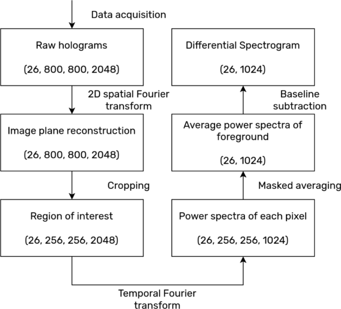
Flowchart of the data processing workflow. The data for each sample undergoes the six data transformation steps outlined. First, 2 d FFT transforms the holograms into reconstructions on the image plane. Next, the data are condensed by cropping around the region of interest (one of the two first-order reconstructions). Next, temporal FFT produces the fluctuation spectra for every pixel. The spectra of the foreground pixels are then averaged. Finally, the log-difference of every spectrum is computed with respect to the averaged baseline spectrum. The numbers in the parentheses in each box indicates the shape of the data, in the order of (number of measurements, pixels in x, pixels in y, number of frames).
The data workflow yields a series of power spectra for each well, as shown in Fig. 4a, and a 2D projection of the same data can be seen in Fig. 4b. In these figures, a snapshot of the dynamics are obtained in the form of a fluctuation spectrum at 1 hour intervals. The changes in the spectra are typically small fractions of the overall spectral weight for a given frequency. Therefore, a log-difference between each spectrum and the log-mean of the baseline spectra was computed. \(S_\text {baseline}\) in Eq. 3 is the log-mean of the four baseline spectra, and \(S'_i\) is the log-difference between each spectrum \(S_i\) and the baseline, \(S_\text {baseline}\).
This log-difference \(\Delta \log (S)\) of the fluctuation power spectra is shown as a differential spectrogram that displays the differential time evolution of the power spectra with respect to the baseline. An example of a spectrogram is shown in Fig. 4c, and an alternative representation showing the log spectral shifts as curves is shown in Fig. 4d. The Doppler shift frequency spectrum has a direct correspondence to the momentum of the scattering body in the sample. Since the Reynolds number in the cytoplasm is very low, viscous force dominates and there is a direct inverse correlation between the size of the scattering body and its velocity (and hence its Doppler shift frequency). As such, different frequency ranges of the Doppler shift spectrum can be mapped to different lengthscales of the scattering body. For instance, the high-frequency bands above 2 Hz correspond to small, fast-moving vesicle and organelle transport, which relate to metabolism; the mid-frequency bands from about 0.05 Hz to 2 Hz correspond to larger organelle movement, e.g. of the nucleus; and the low-frequency ranges below 0.05 Hz correspond to the motions of the cell membrane, such as endocytosis and cell shape change17. Any external stimuli that can either increase or decrease the level of activity at each lengthscale, in turn, tend to elicit a corresponding change in the spectral weight of the relevant frequency range.

Visualization of the data processing workflow. (a) A 3D visualization of the change in fluctuation spectra of a DLD microcluster infected with 1 kcfu/mL S. enterica over 26 measurements spanning 26 hours. The z-axis indicates the time of data acquisition. The first four power spectra from t = 0 h to t = 4 h hours along the z-axis are the baseline before a treatment (PBS or infection) is applied. The 22 spectra after 0 hours are measured after infection. (b) All 26 power spectra plotted on 2D log-log axes. The time progresses from blue (\(t=0\) h) to red (\(t=26\) h). The direction of spectral shift is indicated by the black arrows. (c) A differential spectrogram. The horizontal and the vertical axes correspond to the x and the z axes of (a). Black line at \(t=0\) h indicates the time of infection. The color scale is the log-difference of the spectral weight, \(\Delta \log (S)\), where red indicates relative increase in the spectral weight, and blue indicates relative decrease. Each line of the contour overlay indicates 0.2 increment in \(\Delta \log (S)\). (d) A plot showing the same information as shown in panel (c). The time progresses from blue (\(t=0\) h) to red (\(t=26\) h), and the black arrows indicate the direction of spectral shift over time.
Results
The change in the intracellular dynamics of the sentinel tissue causes a change in the distribution of Doppler shift frequencies observed in the light scattered off of the tissue. This change is not confined to a specific frequency range, and so a spectrogram is constructed to track the changes across a wide range of frequencies over long timescale (see methods). It is also necessary to examine the spectral patterns at different infection doses to find both the common features and differences between the different infection doses. In previous proof-of-concept work21, an infection response was observed, but only a single high initial infection dose was applied, and dose-dependent differences could not be examined. In this section, the result for a dose-dependent response to E. coli and S. enterica (salmonella) spanning 5 orders of magnitude from very low (100 cfu/mL) to very high (10 million cfu/mL) is examined. This range of values captures typical concentrations of bacteria in the fluids from an infected patient27,28, as well as the maximum carrying capacity of growth media for in-vitro use. A total of 12 independent experiments were performed using E. coli to yield total of 91 replicates across different concentrations, and 8 independent experiments were performed using S. enterica to yield a total of 65 replicates across different concentrations. Some replicates were omitted due to cross contamination.
The trend between the initial bacterial load and the magnitude of change in the signature is shown in Fig. 5a for spectrograms of different initial bacteria concentrations ranging from 100 colony forming units per mL (cfu/mL) to \(10^7\) cfu/mL. There is a strong correlation between the initial concentration of the inoculum and the onset speed of the signature. At all concentrations, a similar red-blue-red pattern across low-mid-high frequency emerges that is distinct from that of the control condition for DLD microclusters treated with sterile phosphase buffer saline (PBS). Fig. 5b shows line plots at select frequencies through the spectrograms. In these figures, the steep onsets in the spectral shift are ordered by initial concentration in decreasing order, and the onsets of each concentration are evenly distributed, which is to be expected because the E. coli concentration in the well follows a logistic growth. The offset in initial concentration by an order of magnitude corresponds roughly to 3.3 doubling cycles, which shifts the delay by just over an hour per ten-fold change in concentration.
To demonstrate that bacterial infection causes the shifts in the fluctuation, the time associated with each point of the spectral shift was adjusted by the exponent of the concentration, with scale factor of 3.32, which corresponds to the number of division cycles needed for the E. coli to grow in concentration by an order of magnitude. Fig 5c shows the time-adjusted spectral shifts at three different values of frequency. The spectral shift curves collapse into a single curve on the adjusted time axis.

Observation of the sentinel effect with DLD microclusters inoculated with E. coli at different concentrations. (a) The spectrograms with (0, 100, 1k, 10k, 100k, 1M, 10M cfu/mL) inoculum concentrations demonstrate the correlation between the bacterial concentration and the strength of the signature. Color scale shows \(\Delta \log (S)\), which is the relative change in the spectral weight with respect to the baseline. Black line marks the time of infection. Each line of contour is separated by 0.2 units of \(\Delta \log (S)\). (b) The spectrograms are grouped into three frequency bands and the average log-difference in the spectral weight for each band are plotted. The time of the onset for each frequency is ordered by the initial concentration with approximately even spacing. (c) The spectrograms are grouped into three frequency bands, and the time is shifted to offset the effect of the initial concentrations (\(\log _2(10)\) hours per order of magnitude), demonstrating the scaling collapse of the spectral shift data.
The spectral shift at different frequencies indicates that even at a low initial bacterial load of 100 cfu/mL there is a significant shift away from the baseline (PBS treatment) as early as 2 hours in the mid-frequency band, and within 7 hours in the high frequency band, as shown in isolation in Fig. 6. A concentration of 100 cfu/mL is a practical value for the bacterial load in the blood sample of a patient who is starting to show signs of sepsis29. This suggests that this method can be applied directly to patient serum samples to obtain a meaningful result rather than waiting for the bacteria first to be isolated and cultured to a significantly higher concentration, which typically adds about 24 hours of delay. A similar examination of S. enterica infection for two initial concentrations is shown in Fig. 7.

Early detection of E. coli. (a) The log-difference of the spectral weights in three frequency bands, highlighting only the data for DLD microclusters treated with PBS and those infected by 100 cfu/mL E. coli. The bands and error bars indicate the standard error. The spectral shift observed from the infected microclusters deviates from that observed from the PBS treated microclusters outside the standard error range for the mid-frequency band almost immediately upon infection, reaching a 3 sigma difference as early as 2 hours (red vertical line), and by 7 hours for high-frequency band (blue vertical line). These trends demonstrate the early detection of the effects low dose infection. (b) The tissue-response spectrograms corresponding to the two conditions. Color scale shows the log difference of spectral weight with respect to the baseline. Black line indicates the time of infection. Each of the contour lines are separated by 0.2 units of \(\Delta \log (S)\) on the color scale. The upper panel (DLD + PBS) is the average of 19 replicates, and the lower panel is the average of 8 replicates.

Early detection of salmonella. (a) A differential spectrogram showing the sentinel effect observed in DLD microclusters at two different initial infection doses of S. enterica. Like the E. coli data, the magnitude of the spectral shift is shown to be correlated with the infection dose. Like all the previous figures, the color bar represents the relative change in spectral weight and are supplemented with contour lines at even 0.2 unit spacing. Each panel is an average over N samples, where N is the number of replicates as indicated on each panel. (b>) The corresponding spectral shift plots for three frequency bands. The infected and uninfected conditions are separated beyond standard error range, and the infection signatures appear in order of increasing concentration as expected.
To rule out the possibility that the observed effects in Figs. 5-7 are attributable to the increased backscatter from the motile bacteria, which also increases the opacity, a negative control experiment was devised to differentiate between signals arising from the disruptions in intracellular mechanisms of the infection host relative to signals from increased light scatter due to the proliferating bacteria. The experiment consisted of four distinct conditions: 1) fresh DLD targets washed with sterile PBS (healthy negative control); 2) inactive DLD targets prepared using 10% neutral-buffered formalin (NBF) and treated with sterile PBS (inactive negative control); 3) inactive DLD targets treated with 1000 cfu/mL of S. enterica (inactive positive control to measure direct light scattering); and 4) fresh DLD targets treated with 1000 cfu/mL of S. enterica (healthy positive condition). Weak formalin treatment induces minor cross-linking of proteins and shuts down most intracellular activities in the sample. This allowed a separate examination of the effects of bacterial activities in and around the microclusters without a response from the infected host tissue. The tissue samples treated with 10% NBF were rinsed multiple times with PBS to remove any residual formalin that can affect the bacteria. By measuring the difference between the signals from these four conditions, the signatures arising solely from the tissue response to the infection are isolated from the other effects. The spectrograms for these four conditions are shown in Fig. 8.
In Fig. 8a, the two PBS treated targets show a notable difference. The Fresh DLD microclusters that were given a dose of sterile PBS show gradual enhancement of the low frequencies (red-shift), which is associated with decreasing cell metabolism30, likely due to exhaustion of food and increasing metabolic byproduct in the well. On the other hand, the microclusters that were treated with NBF before the experiment show no such trend, presumably because in its cross-linked state, the cells in the tissue have low metabolic activity. When comparing between the NBF-treated tissue that was given sterile PBS, and the NBF-treated tissue that was given a 1000 cfu/mL dose of S. enterica suspended in PBS, there is a gradual and pronounced increase in the very low frequency range in the spectrogram of the infected tissues that is absent in the spectrogram of uninfected ones. Because the tissue itself is unable to respond in any significant way to the infection (since it is weakly cross-linked), the observed difference can be attributed to the motility of the bacteria themselves.
In the last comparison, between the fresh DLD microclusters that were infected with S. enterica, and the NBF-treated DLD microclusters that were infected, there is a pronounced suppression of the mid-frequencies and an enhanced high-frequencies in the former condition, that are notably absent in the latter. Because the only difference between the two conditions is the metabolic viability of the sentinel tissues themselves, the observed difference is attributable to the interaction between the bacteria and the infecting host, i.e. it is attributed to the tissue’s response to the infection, rather than the mere presence of motile bacteria in the field of view.

Negative control to examine signals solely from the activities of motile bacteria. (a) Averaged differential spectrograms showing the effects of four different conditions on the fluctuation spectra of DLD microclusters. The top left panel shows fresh targets treated with PBS applied after the baseline time of 4 hours; top right panel shows formalin washed targets treated with PBS solution; bottom left panel shows formalin-washed targets infected with 1000 cfu/mL; bottom right panel shows fresh target infected with 1000 cfu/mL of salmonella. The 4 hour mark is indicated by the black horizontal line. Measurements before the 4 hours mark establish the baseline spectrum for each sample, which is used to compensate for the extrinsic variability between samples. The color scale on each plot visualizes the relative change in the spectral weight with respect to the baseline. The contour lines are set at 0.2 unit interval of \(\Delta \log (S)\). Each panel is the average over N replicates, where N is the number as noted on each panel. (b) Normalized spectral density difference of microclusters infected with S. enterica compared to PBS treatment, over three different frequency bands. Translucent bands and the bars show standard error for the spectral density shifts. Dotted black line shows the growth curve for the concentration of S. enterica over the same period of time, starting from 1 kcfu/mL. The details of how the concentration curve was obtained and calibrated can be found in the Information S3.
The differences among the four conditions are especially pronounced when looking at the individual line plots for different frequencies, as shown in Fig. 8b. The differential spectral densities of both the NBF-treated and fresh tissue show changes in the 0.1 and 0.3 Hz plots, though the signal from NBF-treated tissue is much weaker. On the other hand, at 4.3 and 11.85 Hz (high frequency), there is no discernable signal from any condition except the fresh DLD infected with S. enterica. These results suggest that while the free swimming bacteria do contribute to the signal, the signal that is observed upon infection can be attributed to the response of the tissue sentinel to the infection, reinforcing the validity of the “sentinel effect” as a surrogate observable for bacterial infection.
Conclusion
In this paper, we presented the case for the use of common-path, long-coherence form of biodynamic imaging (BDI) for early detection of bacterial infection. To accomplish this, we used DLD-1 microclusters, which are in vitro organoids, as infection sentinels whose physiological response to infection, which we call the sentinel effect, is used as a surrogate observable for the presence of bacteria. Our results show that using this method, the sentinel effect can be detected within about 7 hours after infection even with initial dose as low as 100 \(\mu\)L of 100 cfu/mL, which is approximately 10 individual bacteria. As this falls within the range of bacterial concentrations found in patients showing early signs of sepsis, it is conceivable that patient fluid sample such as blood could be used with minimal preparation, rather than having to wait 18–24 hours or more to isolate and culture the bacteria, which is the norm in clinical standards10. Note that while growing the DLD microclusters take 3–5 days in the incubator, the microclusters can be grown in advance without waiting for the patient sample, much like how agar plates can be prepared in advance before bacteria is inoculated, and therefore the preparation time for the DLDs is not included in the estimation of the time to detection.
We have also demonstrated that the sentinel effect is distinct from the dynamic signals arising from the run-and-tumble motion of the motile bacteria, as the same distinct signal did was absent when the tissue was pre-treated with 10% neutral-buffered formalin, which cross-links the proteins in the tissue and renders it unable to respond to any stimuli. This suggests that the important factor is the tissue’s response to the presence of the bacteria, rather than merely the presence of bacteria itself.
In the future, we plan to push this method of measuring bacterial infection in the direction of antimicrobial susceptibility testing (AST) on bacteria. The technique has a competitive advantage, as we can simply watch for the suppression of the sentinel effect in the presence of antibiotics, using a protocol very similar to one presented here, as opposed to culturing the isolated bacteria and running a disk diffusion test, which can take on the order of days10 rather than hours.
Discussion
The canary in the coal mine was an early example of a living biosensor, also known as a sentinel species, first proposed in 1895 by the eccentric British physiologist J. S. Haldane to detect carbon monoxide31. Coal miners began carrying canaries down into coal mines as early as 1896, and the practice continued up to the late 20th century. The concept of a sentinel is that a small and sensitive organism exhibits modified behavior (death in the case of the canary) before the macroscopic detection of an adverse effect was possible. Bacterial pathogens, likewise, might be detected by leveraging their influence on the intracellular dynamics of a tissue sentinel before the macroscopic effects of the bacteria can be detected directly.
For instance, light scattering from a bacterium in the near infrared is in the Rayleigh-Mie cross-over regime because the typical scale of the microbe is a sizable fraction of the wavelength of light. This sets the scattering cross section to be a fraction of the cross-sectional area of the object. Hence, for a typical incident intensity of 10 mW/cm\(^2\) the scattered power from a single bacterium is in the range of 100 fW scattered into a \(4\pi\) solid angle. A collecting objective might capture 1% of the solid angle to yield 1 fW of detectable power at a photodetector. For a silicon photodetector noise- equivialent power (NEP) of 10 pW per root Hertz, this would require 10,000 bacteria to be in the scattering volume, and for a microliter volume this is a target concentration of 10\(^7\) cfu/mL with a mass density of about 10 \(\mu\)g/mL32. If the starting concentration is 100 cfu/mL with a doubling time of 20 minutes, as a rough estimate this would require around 9 to 10 hours before detectable light scattering can occur.
Conversely, a single bacterium can modify the intracellular dynamics of a living cell in a tissue culture. A tissue micro-cluster containing 10,000 cells has a diameter of approximately 300 microns and a volume of 10 \(\mu\)L. Assuming that the effect of a single bacterium can be detected within a group of 10 sentinel cells (approximately a 10% limit of detection (LOD) using biodynamic imaging33), this corresponds to \(10^5\) cfu/mL which could be attained in about 6 hours beginning with an inoculation of 100 cfu/mL. Hence a living tissue sentinel can, in principle, provide a therapeutic “window” of 2 to 3 hours before light scattering can be detected directly from the proliferating bacteria. The sensitivity of biodynamic imaging to intracellular dynamics originates from its ability to maximize speckle contrast by relaxing spatial resolution and hence enabling larger scattering contributions per resolution voxel. The spatial resolution of common path BDI is between 10 and 20 microns laterally, but with no ability to resolve features axially. This is due to the long coherence of the light source used, which effectively projects all holographic reconstructions along the axial direction in one 2D image, resulting in a flattened volume. In practice, the microcluster samples used were relatively thin (50–100 microns) and so the lack of axial resolution was not a significant limitation. All in all, each pixel, which represents a volume of about 20 \(\mu\)m \(\times\) 20 \(\mu\)m \(\times\) 50–100 \(\mu\)m, is estimated to contain about 2–5 bacteria, which is far below what could be detected using conventional imaging methods when the bacteria are obscured by the tissue.
In previous work, biodynamic imaging demonstrated that bacterial infections could be detected in living sentinels21, but the inoculation concentrations were very high in the range from \(10^5\) cfu/mL to \(10^7\) cfu/mL. These high concentrations presented no challenge to detection limits and the sentinel targets were large tumor spheroids. However, to have clinical utility, the biodynamic sentinel assay must operate with clinically relevant inoculation concentrations and must achieve detection within hours. This required the substantial change in the biodynamic protocols which are described in detail in this paper. The size of the tissue sentinels was reduced from 500 micron diameters to 200 micron diameter to increase surface-to-volume ratios. The coherence gate was removed by converting to a long-coherence light source to probe larger volumes, and a common-path configuration was adopted to reduce sensitivity to mechanical noise and hence increase the detection sensitivity. These three alterations (sentinel size, coherence length, and common-path configuration) significantly improved the detection sensitivity to enable inoculation with 100 cfu/mL which is a clinically relevant concentration.
Changes in the biodynamic spectrograms were observed within as little as 2 hours after inoculation at 100 cfu/mL at the low-frequency range, with statistically significant effects across the broad-band spectrum occurring within 7 hours. These time frames and detection limits are within the estimates discussed above. Validation of the “sentinel window”, i.e. the time span between when the bacterial infection is detected in the intracellular dynamics by BDI and the time when significant light scattering is detected from the bacteria directly, was accomplished by culturing tissue with substantially inhibited intracellular dynamics to act as a positive control. The weak formalin treatment to the tissue prevents significant intracellular transport by partially cross-linking proteins while still allowing the cell tissue to remain alive. Bacterial infection of these tissues has minimal effect on their dynamics, but the proliferation of the bacteria led to eventual direct detection through light scattering. Comparing this positive control against the healthy sentinels, combined with negative control experiments, confirmed the dynamical effects of the bacteria on the intracellular Doppler spectra.
These findings have important implications for the viability of the method in clinical settings. BDI has unique advantages for an infection assay because the specific bacterial strain and mechanism of antibiotic resistance are not required for the protocol to be carried out; it is a strain-agnostic method. This ability to detect the presence of the bacteria while being blind to the type of infection, and with high sensitivity to low concentrations of infecting bacteria, shows promise for the technique to perform as a fast test for infection as well as for antibiotic resistance screening, which is the subject of ongoing research with the sentinel method.
Data availability
The data used to produce the figures in this paper is made available upon request to [email protected].
References
Sanders, J. W., Fuhrer, G. S., Johnson, M. D. & Riddle, M. S. The epidemiological transition: The current status of infectious diseases in the developed world versus the developing world. Sci. Prog.91, 1–37 (2008).
Ikuta, K. S. et al. Global mortality associated with 33 bacterial pathogens in 2019: A systematic analysis for the global burden of disease study 2019. Lancet400, 2221–2248 (2022).
Rudd, K. E. et al. Global, regional, and national sepsis incidence and mortality, 1990–2017: Analysis for the Global Burden of Disease study. Lancet395, 200–211 (2020).
Michael, C. A., Dominey-Howes, D. & Labbate, M. The antimicrobial resistance crisis: Causes, consequences, and management. Front. Public Health2, 145 (2014).
Marshall, B. M. & Levy, S. B. Food animals and antimicrobials: Impacts on human health. Clin. Microbiol. Rev.24, 718–733 (2011).
Mathew, A. G., Cissell, R. & Liamthong, S. Antibiotic resistance in bacteria associated with food animals: A united states perspective of livestock production. Foodborne Pathog. Dis.4, 115–133 (2007).
O’Neill, J. Tackling a crisis for the health and wealth of nations. Review on Antimicrobial Resistance (2014).
Zasowski, E. J. et al. A systematic review of the effect of delayed appropriate antibiotic treatment on the outcomes of patients with severe bacterial infections. Chest 158, 929–938 (2020).
Balouiri, M., Sadiki, M. & Ibnsouda, S. K. Methods for in vitro evaluating antimicrobial activity: A review. J. Pharm. Anal.6, 71–79 (2016).
Schwalbe, R., Steele-Moore, L. & Goodwin, A. C. Antimicrobial susceptibility testing protocols (Crc Press, 2007).
Webber, D. M., Wallace, M. A. & Burnham, C.-A.D. Stop waiting for tomorrow: disk diffusion performed on early growth is an accurate method for antimicrobial susceptibility testing with reduced turnaround time. Journal of clinical microbiology 60, e03007-20 (2022).
Zasowski, E. J., Claeys, K. C., Lagnf, A. M., Davis, S. L. & Rybak, M. J. Time is of the essence: The impact of delayed antibiotic therapy on patient outcomes in hospital-onset enterococcal bloodstream infections. Clin. Infect. Dis.62, 1242–1250 (2016).
Ortega, F. E., Koslover, E. F. & Theriot, J. A. Listeria monocytogenes cell-to-cell spread in epithelia is heterogeneous and dominated by rare pioneer bacteria. Elife 8, e40032 (2019).
Demchenko, A. P. Photobleaching of organic fluorophores: quantitative characterization, mechanisms, protection. Methods and applications in fluorescence 8, 022001 (2020).
Kirchhoff, J. et al. Simple ciprofloxacin resistance test and determination of minimal inhibitory concentration within 2 h using raman spectroscopy. Anal. Chem.90, 1811–1818 (2018).
Chen, C. & Hong, W. Recent development of rapid antimicrobial susceptibility testing methods through metabolic profiling of bacteria. Antibiotics10, 311 (2021).
Nolte, D. D. Coherent light scattering from cellular dynamics in living tissues. Reports on Progress in Physics 87, 036601 (2024).
Leitgeb, R. A., Werkmeister, R. M., Blatter, C. & Schmetterer, L. Doppler optical coherence tomography. Prog. Retin. Eye Res.41, 26–43 (2014).
Huang, S. et al. In vivo imaging of retinal hemodynamics with oct angiography and doppler oct. Biomed. Opt. Express7, 663–676 (2016).
Thouvenin, O., Grieve, K., Xiao, P., Apelian, C. & Boccara, A. C. En face coherence microscopy. Biomedical optics express 8, 622–639 (2017).
Choi, H. et al. Doppler imaging detects bacterial infection of living tissue. Communications Biology 4, 178 (2021).
Edwards, C., Bhaduri, B., Griffin, B., Goddard, L. & Popescu, G. Epi-illumination diffraction phase microscopy with white light. Opt. Lett.39, 6162–6165 (2014).
Finkeldey, M., Göring, L., Brenner, C., Hofmann, M. & Gerhardt, N. C. Depth-filtering in common-path digital holographic microscopy. Opt. Express25, 19398–19407 (2017).
Jeong, K., Lopera, M. J., Turek, J. J. & Nolte, D. D. Common-path interferometer for digital holographic doppler spectroscopy of living biological tissues. J. Biomed. Opt.26, 030501–030501 (2021).
Saleh, B. E. & Teich, M. C. Fundamentals of photonics, 2 volume set (john Wiley & sons, 2019).
Li, Z. et al. Tissue dynamics spectroscopic imaging: Functional imaging of heterogeneous cancer tissue. J. Biomed. Opt.25, 096006–096006 (2020).
Capdevila, J. et al. Value of differential quantitative blood cultures in the diagnosis of catheter-related sepsis. Eur. J. Clin. Microbiol. Infect. Dis.11, 403–407 (1992).
Dietzman, D. E., Fischer, G. W. & Schoenknecht, F. D. Neonatal escherichia coli septicemia—bacterial counts in blood. The Journal of pediatrics 85, 128–130 (1974).
Yagupsky, P. & Nolte, F. S. Quantitative aspects of septicemia. Clin. Microbiol. Rev.3, 269–279 (1990).
Hua, Z. et al. Comparative oncology chemosensitivity assay for personalized medicine using low-coherence digital holography of dynamic light scattering from cancer biopsies. Scientific Reports 14, 2760 (2024).
Haldane, J. The action of carbonic oxide on man. J. Physiol.18, 430 (1895).
Mira, P., Yeh, P. & Hall, B. G. Estimating microbial population data from optical density. PLoS One17, e0276040 (2022).
Li, Z. et al. Doppler fluctuation spectroscopy of intracellular dynamics in living tissue. J. Opt. Soc. Am. A Opt. Image Sci. Vis.36, 665–677 (2019).
Acknowledgements
This work was carried out with support from CBET grant NSF-2200186.
Author information
Authors and Affiliations
Contributions
D.L. performed experiments, analysis, and wrote the manuscript. Z.H. performed experiments. F.C. and J.T. prepared the biological samples used in the experiments. M.L. and D.N. supervised the project. All authors reviewed the manuscript.
Corresponding author
Ethics declarations
Competing interests
J.T. and D.N. are stakeholders in Animated Dynamics, a company that commercializes the biodynamic imaging technique discussed in the paper. Other authors declare no competing interests.
Additional information
Publisher’s note
Springer Nature remains neutral with regard to jurisdictional claims in published maps and institutional affiliations.
Supplementary Information
Rights and permissions
Open Access This article is licensed under a Creative Commons Attribution-NonCommercial-NoDerivatives 4.0 International License, which permits any non-commercial use, sharing, distribution and reproduction in any medium or format, as long as you give appropriate credit to the original author(s) and the source, provide a link to the Creative Commons licence, and indicate if you modified the licensed material. You do not have permission under this licence to share adapted material derived from this article or parts of it. The images or other third party material in this article are included in the article’s Creative Commons licence, unless indicated otherwise in a credit line to the material. If material is not included in the article’s Creative Commons licence and your intended use is not permitted by statutory regulation or exceeds the permitted use, you will need to obtain permission directly from the copyright holder. To view a copy of this licence, visit http://creativecommons.org/licenses/by-nc-nd/4.0/.
About this article

Cite this article
Lim, D., Hua, Z., Cunha, F.d. et al. Intracellular doppler spectroscopy of live tissue sentinels for a fast in-vitro bacterial infection assay. Sci Rep 15, 24020 (2025). https://doi.org/10.1038/s41598-025-08523-z
Received:
Accepted:
Published:
DOI: https://doi.org/10.1038/s41598-025-08523-z
